Anatomy of hierarchy: feedforward and feedback pathways in macaque visual cortex

Abstract

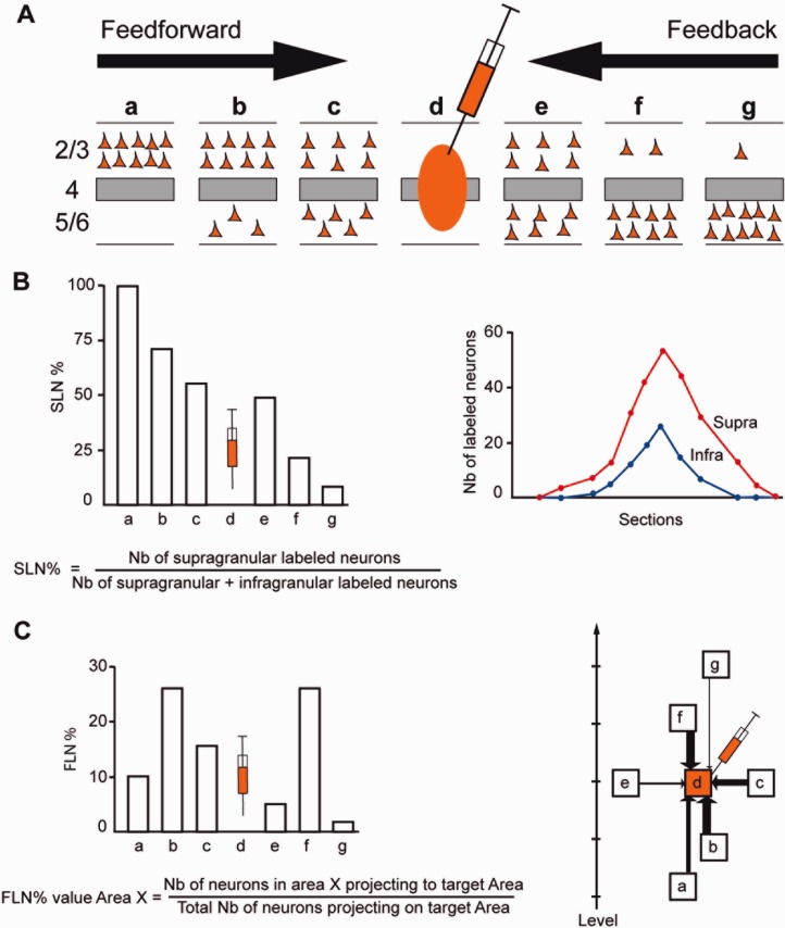
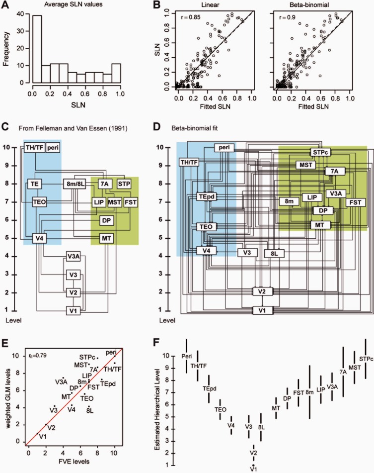
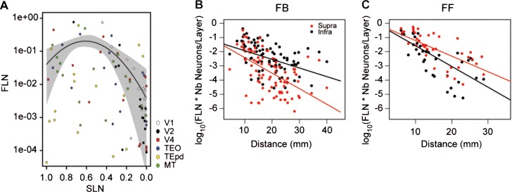
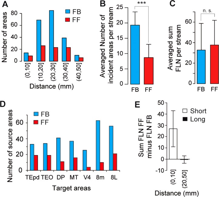
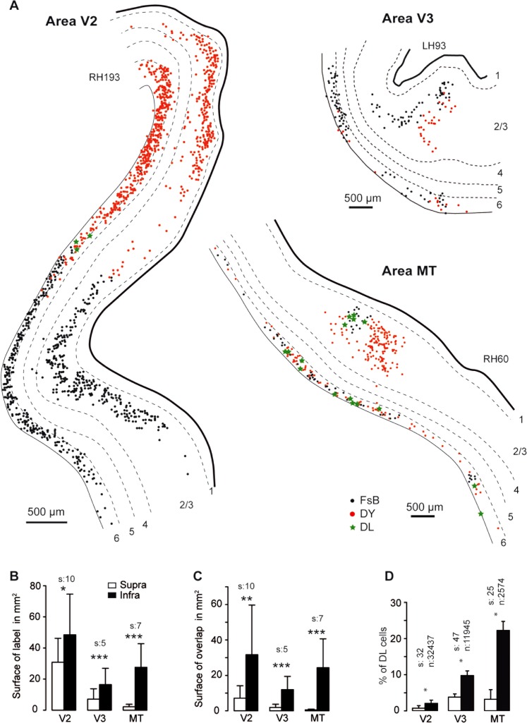
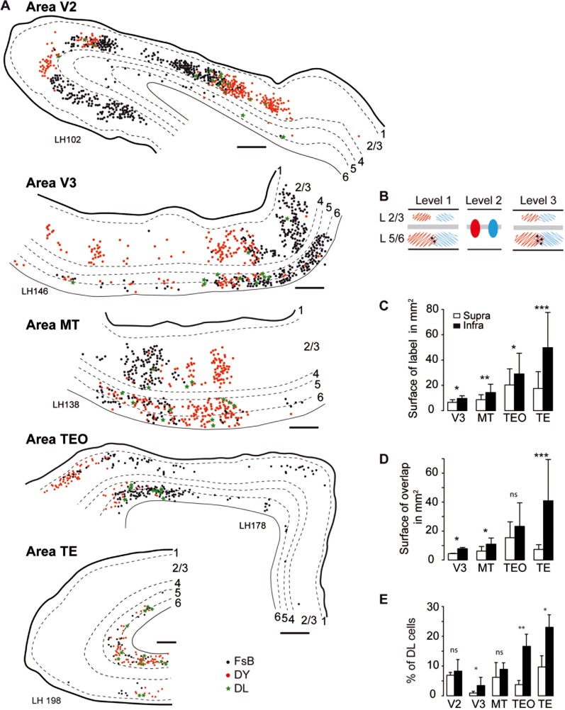
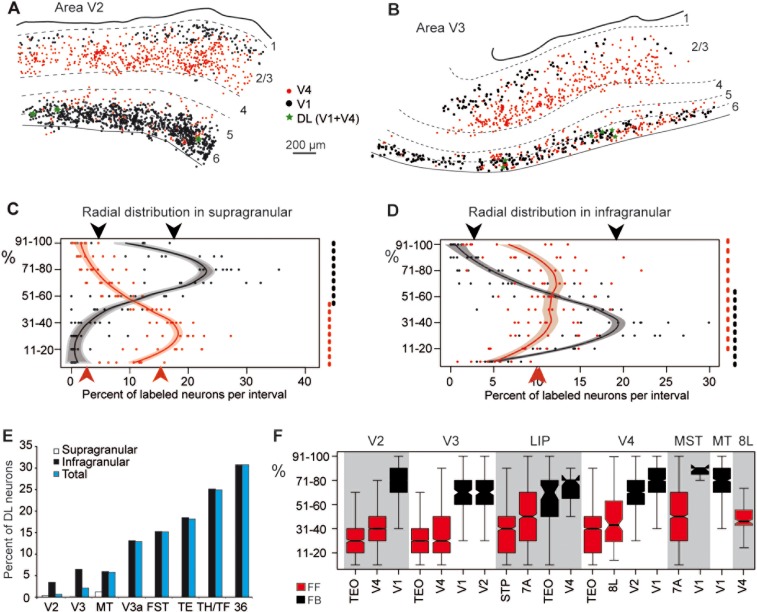
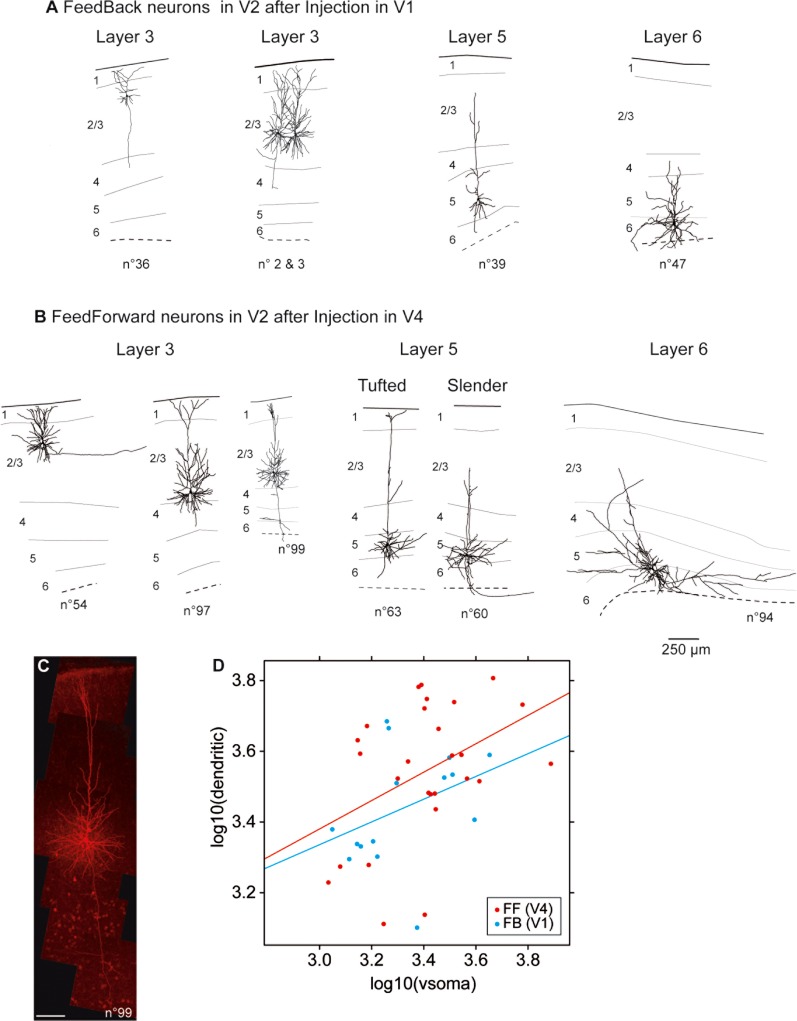
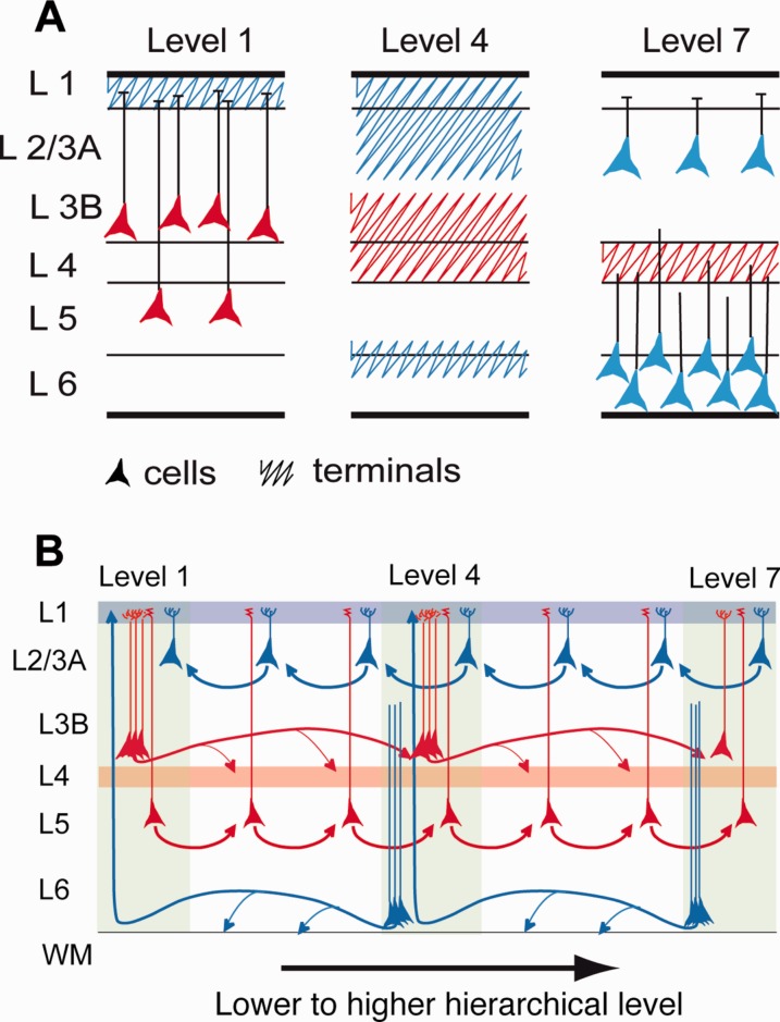
The laminar location of the cell bodies and terminals of interareal connections determines the hierarchical structural organization of the cortex and has been intensively studied. However, we still have only a rudimentary understanding of the connectional principles of feedforward (FF) and feedback (FB) pathways. Quantitative analysis of retrograde tracers was used to extend the notion that the laminar distribution of neurons interconnecting visual areas provides an index of hierarchical distance (percentage of supragranular labeled neurons [SLN]). We show that: 1) SLN values constrain models of cortical hierarchy, revealing previously unsuspected areal relations; 2) SLN reflects the operation of a combinatorial distance rule acting differentially on sets of connections between areas; 3) Supragranular layers contain highly segregated bottom-up and top-down streams, both of which exhibit point-to-point connectivity. This contrasts with the infragranular layers, which contain diffuse bottom-up and top-down streams; 4) Cell filling of the parent neurons of FF and FB pathways provides further evidence of compartmentalization; 5) FF pathways have higher weights, cross fewer hierarchical levels, and are less numerous than FB pathways. Taken together, the present results suggest that cortical hierarchies are built from supra- and infragranular counterstreams. This compartmentalized dual counterstream organization allows point-to-point connectivity in both bottom-up and top-down directions.

Keywords: cell morphology; monkey; neocortex; retrograde tracing.

Figure 1

Quantitative parameters characterizing the hierarchy. A: The laminar distribution of parent neurons in each pathway, referred to as SLN (fraction of supragranular neurons) is determined by high-frequency sampling and quantitative analysis of labeling. Supra- and infragranular layer neurons contribute to both FB and FF pathways, and their relative proportion is characteristic for each type of pathway. For a given injection there is a gradient of SLN of the labeled areas, between purely FF (SLN = 100%, all the parent neurons are in the supragranular layers) to purely FB (SLN = 0%, all the parent neurons in the infragranular layers) and a spectrum of intermediate proportions. B: All labeled areas can then be ordered by decreasing SLN values and this order is consistent with hierarchical order according to Felleman and Van Essen (1991). SLN is thus used as an indicator of hierarchical distance between areas from the same injection (Barone et al., ; Vezoli et al., 2004). C: FLN (fraction of labeled neurons) indicates the relative strength of each pathway (in number of labeled neurons) compared to the total number of neurons that are labeled in the cortical hemisphere after the injection. It requires counting labeled neurons from sections spanning the whole brain, but gives insight into the weight of connections. Vezoli et al. (2004) showed that short-distance connections have high FLN values, whereas the strength of connection decreases as physical distance between source and target areas increases.

Figure 2

Laminar limits of area V2.

Figure 3

A: Schematic illustration of linear model of relation of SLN to hierarchical level. Relative hierarchical scale values depend directly on the difference of SLN values. For a given injection in two hypothetical areas, hierarchical distance is a linear function of SLN. The difference in hierarchical level maps onto a fixed SLN difference in each injection, indicated by the difference between each red dashed and blue dotted line as projected on the SLN scale axis for the hypothetical areas A1 and A2. B: Pairs plots: a set of scatterplots showing the correlation between SLN values obtained in common source areas labeled from specific pairs of injected areas (as indicated along the diagonal). Each point represents the average pair of SLN values obtained in a single source area. The blue dashed lines are the “best fit” lines of unit slope. The solid lines are the “best fit” lines that dually minimize distance from the points in both axes. C: Correlation matrices from the pairs plots of raw SLN values.

Figure 4

A: Schematic illustration of probit model of the relation of SLN to hierarchical level. Hierarchical scale values depend on SLN values through a sigmoidal transformation, here given by a probit (inverse cumulative Gaussian) transformation. A fixed hierarchical distance between hypothetical areas A1 and A2 corresponds to different SLN differences, depending on the injection. Conversely, small differences near extreme FB or FF values (0 and 1, respectively) can translate into the same hierarchical distances as larger SLN differences for more lateral connections. B: Pairs plots between probit-transformed SLN values of common areas from different injections. Conventions are otherwise the same as for the pairs plots in Figure 3B. C: Correlation matrices from the pairs plots of probit transformed SLN values. Ventral stream areas display high positive correlations, which seem to be accentuated by the probit transform.

Figure 5

A: Frequency distribution of SLN values. B: Relation between the observed and predicted SLN from the linear and beta-binomial models C: Model of hierarchy of visual areas derived from Felleman and Van Essen (1991). D: Model of hierarchy of visual areas built form SLN and FLN values shown in Table 2. Blue background ventral stream areas; green background dorsal stream areas. E: Correlation of the hierarchy shown in (C,D). F: Estimated hierarchical levels from the beta-binomial model with 95% confidence intervals for the estimated values.

Figure 6

Combinatorial distance rule determines the SLN of FF and FB projections. A: Relationship of FLN to SLN. The curve is the best fitting parabola and the gray envelope indicates the standard errors of the fit. B: FB projections, fit with a linear model to the supra- and infragranular layer fractions of the FLN. This figure is generated based on injections in nine areas (V1, V2, V4, DP, TEO, TEpd, STPc MT, and 7A).The prefrontal areas were excluded from the source and target list due to their tendency to overrun the distance and hierarchy rules. The lines are constrained to have a common intercept at the origin. The constrained fit did not differ significantly from an unconstrained fit in which independent intercepts were permitted (F(1, 172); 0.40; P = 0.53). C: Same analysis as in (B) for the FF projections. Again, constrained fit did not differ significantly from unconstrained fit (F(1, 74) = 0.86, P = 0,31).

Figure 7

Influence of distance from target area on FF and FB pathways (target areas V1, V2, V4, DP, MT, TEpd, TEO, STPc, 7A, 8L, 8m). A: Incidence of FF (100% ≥ SLN% ≥ 55%) and FB (0% ≤ SLN% ≤ 45%) at different distance intervals. B: Comparison of the average numbers of FF and FB pathways for each target area. C: Average across injections of the sum of FLN in FF and FB pathways. D: Incidence of FF and FB in middle hierarchy areas. Conventions as in (A). E: Influence of distance on FLN magnitude. For each target area we subtracted the sum total FLN% of FB projections from the sum total FLN% of FF projections. The histogram represents the median of the result. Error bars: median absolute deviation, short distance 0–10 mm, long 20–50 mm.

Figure 8

Topography of projections to area V1. A: Spatial layout of FB neurons in supra- and infragrauluar layers of extrastriate areas following dual injections in area V1. B: Histograms showing surface area of projection zones. C: Overlap surface of the projection zones of both dyes. D: Percentage of double-labeled neurons in overlap zone in B. FsB, Fast blue; DY, Diamidino yellow; DL, double labeled; s = numbers of sections, n = number of neurons. ***P 0.001, **P 0.01, *P 0.05.

Figure 9

Spatial extent, overlap, and proportions of double-labeled neurons in extrastriate areas following dual injections of area V4. A: Charts of labeled neurons in extrastriate areas following dual injections in area V4. B: Schematic representation. C: Surface area in mm² (number of sections for reconstructions: V3 = 6, MT = 9, TEO = 4, TE = 6). D: Surface area in mm² of the overlap zone of FB and DY labeled neurons (number of sections as in C). E: Percentage of double-labeled neurons (V2 number of sections = 58, neurons = 13,231; V3 sections = 12, neurons = 6773; MT sections = 13, neurons = 3352; TEO sections = 3, neurons = 1971; TE sections = 5, neurons = 2291). Scale bar: 500 μm. FsB, Fast blue; DY, Diamidino yellow; DL, double labeled; empty bars supragranular layers, filled bars infragranular layers. ***P 0.001, **P 0.01, *P 0.05.

Figure 10

Segregation of FF and FB pathways. A,B: Charts of retrograde labeled neurons in a parasagittal section of area V2 (A) and area V3 (B) following injections of DY in area V1 and FsB in area V4. C: Percentage of labeled FF and FB neurons per depth bin in supragranular layers of extrastriate cortex (areas V2, V3, V4, LIP, MST, MT). Envelope corresponds to a loess predicted distribution. Black dashed line indicates the FB compartment identified by a tree model; the high and low mean for neuronal distribution within and outside the compartment are indicated by black arrowheads. Red dashed line identifies the FF compartment isolated by tree model, the red arrowheads indicate the high and low mean for neuronal distribution within and outside the compartment. D: The segregation of FF and FB neurons in the infragranular layers. Same conventions as in (C). E: Laminar distribution of double labeled neurons in visual areas V2, V3, V3a, MT, FST, TE, TH/TF, area 36. Proportions of double-labeled neurons expressed as percentages of the smallest population of single-labeled neurons. F: Boxplots of the distribution of neurons in supragranular layers for individual projection pathways. C,F: Ordinate scale goes from 0 top of layer 4, 100 bottom of layer 1. D: 0 bottom of layer 6, 100 top of layer 5. DL, double-labeled.

Figure 11

Morphology of projection neurons in V2. A,B: Area V2 cell morphology of parent neurons of interareal pathways. C: Photomontage reconstruction of an FF neuron in layer 3B shown in B. D: Scatterplot of cell soma size and dendritic arbors. Scale bars = 250 μm in A,B; 100 μm in C.

Figure 12

Organization of FB and FF pathways. A: Influence of distance on the distribution of parent neurons (Kennedy and Bullier, ; Perkel et al., ; Van Essen et al., ; Kennedy et al., ; Sousa et al., ; Rockland et al., ; Rockland and Van Hoesen, ; Barone et al., 2000). Influence of distance on distribution of terminals (Tigges et al., , ; Rockland and Pandya, ; Henry et al., ; Rockland and Drash, ; Anderson and Martin, 2006). FF level 1 neurons project to layer 4 and layer 3B in level 4 and layer 4 of level 7. FB layer 2/3A neurons in level 7 project to layers 1, 2/3A in level 4 and layer 1 of level 1. Level 7 layer 6 FB neurons project to layer 6 in level 4 and layer 1 of level 1. B: Long-distance FF pathway in layer 3B, tightly integrated with layer 4 via basal dendrites and the targeting of layer 4 of upstream areas. Long-distance FB pathway in layer 6 targeting layer 6 of adjacent areas and layer 1 of far-distant downstream areas (Rockland and Van Hoesen, 1994). In the layer 2/3A there is a short-distance FB pathway tightly integrated with layer 1 via apical dendritic tufts. In layer 6 there are two short-distance FF pathways in layer 5 and 6, the layer 5 pathway being in contact with layer 1 via its apical dendrites. The parent populations of FF and FB are highly distinct, and neurons very rarely have FF and FB collaterals.

References

1. Anderson JC, Martin KA. Synaptic connection from cortical area V4 to V2 in macaque monkey. J Comp Neurol. 2006;495:709–721. - PubMed
1. Anderson JC, Binzegger T, Martin KA, Rockland KS. The connection from cortical area V1 to V5: a light and electron microscopic study. J Neurosci. 1998;18:10525–10540. - PMC - PubMed
1. Anderson JC, Kennedy H, Martin KA. Pathways of attention: synaptic relationships of frontal eye field to v4, lateral intraparietal cortex, and area 46 in macaque monkey. J Neurosci. 2011;31:10872–10881. - PMC - PubMed
1. Angelucci A, Bressloff PC. Contribution of feedforward, lateral and feedback connections to the classical receptive field center and extra-classical receptive field surround of primate V1 neurons. Prog Brain Res. 2006;154:93–120. - PubMed
1. Barbas H. Pattern in the laminar origin of corticocortical connections. J Comp Neurol. 1986;252:415–422. - PubMed
Publication types
LinkOut - more resources