Measurement and modeling of transcriptional noise in the cell cycle regulatory network

Abstract

Fifty years of genetic and molecular experiments have revealed a wealth of molecular interactions involved in the control of cell division. In light of the complexity of this control system, mathematical modeling has proved useful in analyzing biochemical hypotheses that can be tested experimentally. Stochastic modeling has been especially useful in understanding the intrinsic variability of cell cycle events, but stochastic modeling has been hampered by a lack of reliable data on the absolute numbers of mRNA molecules per cell for cell cycle control genes. To fill this void, we used fluorescence in situ hybridization (FISH) to collect single molecule mRNA data for 16 cell cycle regulators in budding yeast, Saccharomyces cerevisiae. From statistical distributions of single-cell mRNA counts, we are able to extract the periodicity, timing, and magnitude of transcript abundance during the cell cycle. We used these parameters to improve a stochastic model of the cell cycle to better reflect the variability of molecular and phenotypic data on cell cycle progression in budding yeast.

Keywords: Saccharomycescerevisiae; cell cycle; gene expression noise; single mRNA FISH; stochastic modeling.

Figure 1. Summary of single mRNA FISH method and mRNA distributions. (A) Schematic of how the FISH probes hybridize to target mRNAs. (B) Example image showing individual mRNA molecules. Image is a maximum intensity projection of a z-series with merged phase-contrast and fluorescence channels. (C) Detected single transcripts. The image in the left panel was processed as described in “Materials and Methods” to detect spots of single mRNAs. Scale bar = 5 µm. (D) Experimental distributions of mRNA for 16 cell cycle genes. Gray bars show the experimental histograms; red lines are the fit to a single component Poisson, and blue lines are the fit to a two-component Poisson. Data are from the biological replicate shown in Table 1. Similar results were obtained in 2 other biological replicates (Table S1).

Figure 2. Correlation between the timing and magnitude of gene expression from FISH experiments and Cyclebase microarray experiments. (A) CLB2 microarray data plotted on a linear scale with the minimum value set at 0 and the maximum set at 1. Used as an example of how we measure the length of time that the transcript level is greater than the half-maximum level (FWHM, full-width at half maximum). (B) CLB2 microarray data on a log₂ scale. Values are relative to the time-course mean. Used as an example of how we measure the peak:mean value and the total cell cycle time. (C) Correlation plot for each cell cycle gene showing fraction of the high expression population from FISH experiments (1 − β) compared with the fraction of cell cycle time in which transcript levels exceed FWHM level from Cyclebase. (D) Correlation plot for each periodic cell cycle gene showing the ratio of the mean transcript values of the high abundance population (λ₂) to the mean for the population from FISH experiments compared with the peak:mean values from Cyclebase. Data are from the biological replicate shown in Table 1. Similar results are obtained with all biological replicates. Values for CLB2 and SIC1 are not included (see text). Some genes have two peaks of expression in the Cyclebase data, producing two data points. R² values and P values from ANOVA statistical analysis of the linear regressions are shown. Null hypothesis for the P value is that there is no correlation between the FISH and Cyclebase data.

Figure 3.CLN2 mRNA distribution changes during cell cycle progression. Single mRNA FISH was performed on α-factor synchronized CLN2-GFP cells. These cells were chosen, because CLN2 expression is induced at the START transition and should be low in α-factor arrested cells (G₁). Cells were released from arrest (0 min) and allowed to proceed through the cell cycle. Samples were removed from the culture at the indicated times and processed for FISH, FACS analysis of DNA content, and to determine bud morphology as benchmarks for cell cycle progression. Left panel: CLN2 mRNA cellular abundance distributions as determined by FISH. Also shown are single Poisson distributions (red line) and two-component Poisson distributions (blue line) fitted to the mean mRNA abundances. The Poisson parameters and statistics are provided in Table 2. Middle panel: DNA content as determined by FACS analysis with the proportions of 1N and 2N cells indicated as percentages. Percentages are not 100% because of incompletely stained cells that are not within the peaks. Right panel: the proportion of unbudded (G₁) cells, small-budded (< 1/3 size of mother; S-phase) cells, large-budded cells with one nucleus (G₂/M), and large-budded cells with an elongated nucleus in the neck or in which both mother and bud contain a nucleus (anaphase/telophase).

Figure 4. Correlations of mRNA oscillation amplitudes and abundances to protein. Data for all correlation plots is from Table S3. All protein data are derived from Ball et al. (A) Correlation plot for each periodic cell cycle gene showing mRNA amplitudes from FISH experiments (λ₂ − λ₁) compared with protein oscillation amplitudes. Only genes that showed both mRNA and protein oscillations are included. Black line is the linear regression. (B) Correlation plot of all 16 cell cycle genes, showing the ratio of the mean transcript abundance from FISH experiments to the mean protein abundance, as measured by fluorescence (mean pixel intensity/cell). The linear regression and statistics for the entire set (black), for the constitutive genes only (blue) and for the periodic genes only (red) are shown. (C) Correlation plot of all 16 cell cycle genes. Same as (B), except that instead of the mean mRNA abundance for the population, the mean of the high abundance population (λ₂) is used for the periodic genes. R² values and P values from ANOVA statistical analysis of the linear regressions are shown. Null hypothesis for the P value is that there is no correlation between the FISH and protein data.

Figure 5. mRNA distributions from stochastic simulations of the model compared with observed distributions. (A–C) Comparison of experimentally observed mRNA abundance to simulated distributions for (A) CLN2, (B) NET1, and (C) WHI5. Experimental data are from biological replicates shown in Table 1. Similar results are obtained with all biological replicates.

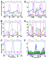
Figure 6. Oscillatory dynamics of key proteins and mRNAs of the model. (A–C) Deterministic simulations of the model showing time-course plots of protein concentrations (A and B) and mRNA abundances (C). (D–F) Stochastic trajectories of the same species are shown as in panels (A–C). In deterministic simulations, cell volume is divided equally at cell division (indicated by the arrows at the bottom of each plot). In stochastic simulations, cell volume is divided 60:40 (mother:daughter) at cell division.

Figure 7. Low mRNA abundance increases cell cycle variability. In these 4 panels we compare the means and coefficients of variation (CV, standard deviation/mean) of 5 cell cycle metrics (T_Div, interdivision time; T_G1, duration of unbudded phase; T_SG2M, duration of budded phase; V_Birth, size at birth; V_Division, size at division) for mother cells and daughter cells. Blue bars, experimental measurements (from ref. 14); green bars, model simulations as described in the text; red bars, model simulations with 4-fold reduction in the average numbers of transcripts of all genes in the model.

References

1. Howell AS, Lew DJ. Morphogenesis and the cell cycle. Genetics. 2012;190:51–77. doi: 10.1534/genetics.111.128314. - DOI - PMC - PubMed
1. Barberis M. Sic1 as a timer of Clb cyclin waves in the yeast cell cycle--design principle of not just an inhibitor. FEBS J. 2012;279:3386–410. doi: 10.1111/j.1742-4658.2012.08542.x. - DOI - PubMed
1. Uhlmann F, Bouchoux C, López-Avilés S. A quantitative model for cyclin-dependent kinase control of the cell cycle: revisited. Philos Trans R Soc Lond B Biol Sci. 2011;366:3572–83. doi: 10.1098/rstb.2011.0082. - DOI - PMC - PubMed
1. Segal M. Mitotic exit control: a space and time odyssey. Curr Biol. 2011;21:R857–9. doi: 10.1016/j.cub.2011.09.023. - DOI - PubMed
1. McInerny CJ. Cell cycle regulated gene expression in yeasts. Adv Genet. 2011;73:51–85. doi: 10.1016/B978-0-12-380860-8.00002-1. - DOI - PubMed
Publication types