Magnetic Resonance Image Example-Based Contrast Synthesis

Abstract

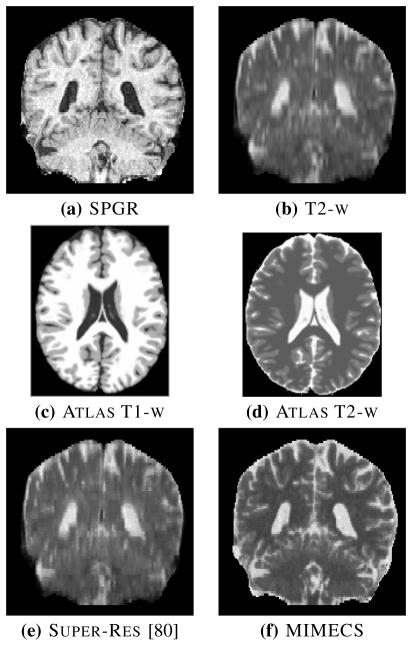
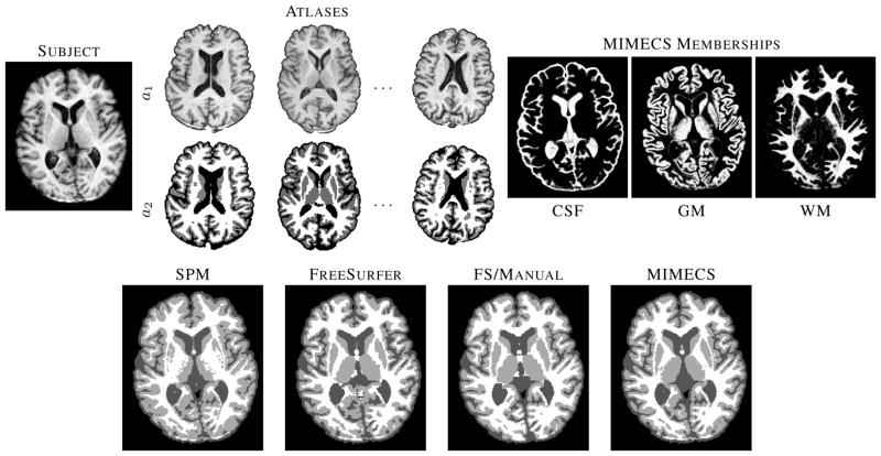
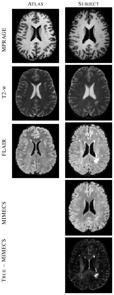
The performance of image analysis algorithms applied to magnetic resonance images is strongly influenced by the pulse sequences used to acquire the images. Algorithms are typically optimized for a targeted tissue contrast obtained from a particular implementation of a pulse sequence on a specific scanner. There are many practical situations, including multi-institution trials, rapid emergency scans, and scientific use of historical data, where the images are not acquired according to an optimal protocol or the desired tissue contrast is entirely missing. This paper introduces an image restoration technique that recovers images with both the desired tissue contrast and a normalized intensity profile. This is done using patches in the acquired images and an atlas containing patches of the acquired and desired tissue contrasts. The method is an example-based approach relying on sparse reconstruction from image patches. Its performance in demonstrated using several examples, including image intensity normalization, missing tissue contrast recovery, automatic segmentation, and multimodal registration. These examples demonstrate potential practical uses and also illustrate limitations of our approach.

Fig. 1

(a) Atlas T1-weighted SPGR and (b) its corresponding T1-weighted MPRAGE. (c) A subject T1-weighted SPGR scan and (d) its T1-weighted MPRAGE image. The atlas SPGR is deformably registered (using SyN [7]) to the subject SPGR. This deformation is applied to the atlas MPRAGE to obtain (e) a synthetic subject MPRAGE. (f) The synthetic MPRAGE image generated by our algorithm, MIMECS.

Fig. 2

An illustration of the MIMECS algorithm. The region of the image labeled A, shows the construction of the atlases A₁ and A₂, see Section III-A for details. Region B shows the input subject images converted into patches b₁(j). Region C denotes the estimation of the coefficients x(j) which relate b₁(j) to the patches of the atlas A₁. Finally, region D shows the computation of the synthetic image ŝ_n+1 by using the learned coefficients x(j) to compute the patch b̂₂(j) based on the atlas A₂. Section III-B describes regions B, C, and D.

Fig. 3. Effect of sparsity of x(j) on the contrast

The left most column shows a subject’s SPGR (top) and MPRAGE (bottom) acquisitions. The second, third, and fourth columns of the top row show synthetic MPRAGEs generated using another portion of the subject’s MPRAGE as the atlas. The synthetic MPRAGEs were generated using λ values of 0.05, 0.80, and 0.95, respectively. The plot shows the MPRAGE synthesis error vs. the average sparsity of all x(j)’s, averaged over all non-zero voxels. The average sparsity scale is on the top of the plot while the sparsity regularization parameter, λ, is plotted on the bottom axis.

Fig. 4

The left column shows images from four (out of fourteen) time-points of a normal BLSA subject, where each image was acquired approximately one year apart. The right column shows synthetic SPGR images, synthesized using MIMECS applied to the corresponding MPRAGE images in the left column.

Fig. 5

GM and ventricle volumes from longitudinal FreeSurfer [71] of a normal subject with 14 scans (first 11 are SPGR, last 3 are MPRAGE).

Fig. 6

(a) Average atlas created using SyN from five BLSA (SPGR) and five OASIS (MPRAGE) images and (b) a zoomed region. (c) Average atlas from five synthetic MPRAGEs from BLSA and five OASIS images (MPRAGE) and (d) a zoomed region. (e) Intensity standard deviation image from SPGR+MPRAGE atlas and (f) intensity standard deviation image from sMPRAGE+MPRAGE atlas.

Fig. 7

(a) Brain volume (GM+WM) and (b) ventricle volume computed using FreeSurfer [74] on 21 normal subjects from the BLSA (SPGR) database and 21 normal subjects from the OASIS (MPRAGE) database, as well as on the 21 synthetic MPRAGEs generated from the BLSA SPGR images.

Fig. 8

(a) and (b) show an atlas pair consisting of MPRAGE and T2-w scans of a normal subject from the Kirby-21 data set. A subject MPRAGE scan (c) is used with MIMECS to synthesize a T2-w image of the subject (d). The acquired subject b₀ image (e) is deformably registered to the subject T1-w image using SyN (with the MI criterion) yielding the corrected image (g). Contours generated from FreeSurfer on the T1-w image (f) are shown on the geometry corrected b₀ image (h). The acquired b₀ image is deformably registered to the synthetic MIMECS image using SyN (CC criterion) to create a MIMECS corrected image (i). Overlaid contours on this image (j) reveal much better geometry correction.

Fig. 9

Coronal views of (a) SPGR (native resolution 0.94 × 0.94 × 1.5mm) and (b) T2-w (native resolution 0.94 × 0.94 × 5mm) scans of a subject. (The T2-w image has been upsampled to the SPGR resolution using trilinear interpolation.) Brainweb (c) T1-w and (d) T2-w phantoms used as an atlas in MIMECS. (e) A hi-res T2-w image upsampled using a non-local super-resolution method. (f) MIMECS synthesized hi-res T2-w image.

Fig. 10

The top row shows a subject T1-w SPGR image, three of the five classification atlases, and fuzzy memberships produced by MIMECS-based tissue classification. Hard segmentations from two leading automatic methods and a manually-corrected method are compared to the hard segmentation of MIMECS.

Fig. 11

The lefthand column contains an atlas for FLAIR synthesis. The righthand column shows the subject’s true images, a synthetic MIMECS FLAIR image, and a subtraction image (true FLAIR minus synthetic MIMECS FLAIR).

References

-
- Bezdek JC, Hall LO, Clarke LP. Review of MR image segmentation techniques using pattern recognition. Med Physics. 1993;20(4):1033–1048. - PubMed
- Bazin PL, Pham DL. Topology-preserving tissue classification of magnetic resonance brain images. IEEE Trans Med Imag. 2007 Apr;26(4):487–496. - PubMed
- Clark KA, Woods RP, Rottenberg DA, Toga AW, Mazziotta JC. Impact of acquisition protocols and processing streams on tissue segmentation of T1 weighted MR images. NeuroImage. 2006;29(1):185–202. - PubMed
- Boesen K, Rehm K, Schaper K, Stoltzner S, Woods R, Lüders E, Rottenberg D. Quantitative comparison of four brain extraction algorithms. NeuroImage. 2004 Jul;22(3):1255–1261. - PubMed
Grants and funding
LinkOut - more resources
Full Text Sources
Other Literature Sources