Compositionality in neural control: an interdisciplinary study of scribbling movements in primates

Abstract

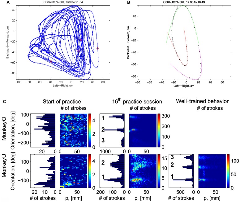
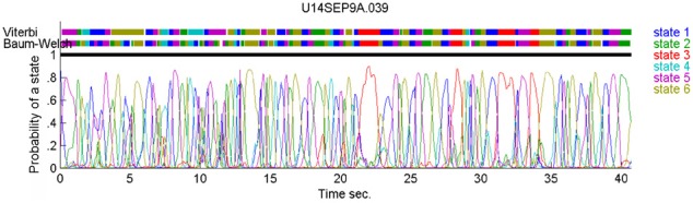
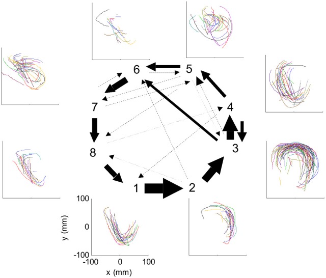
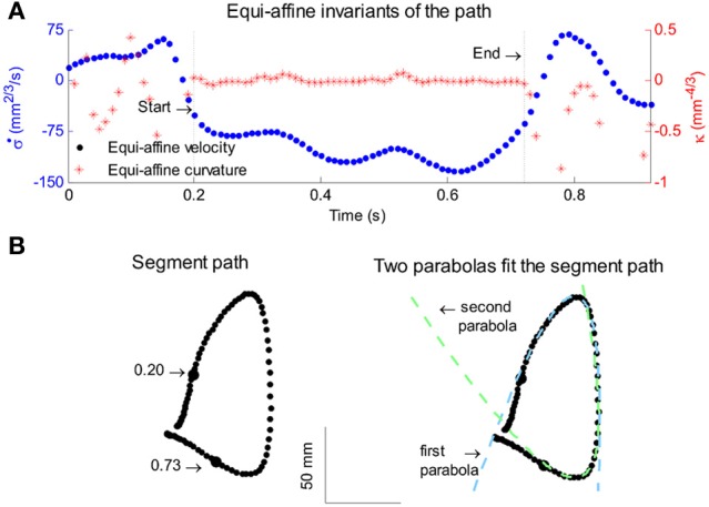
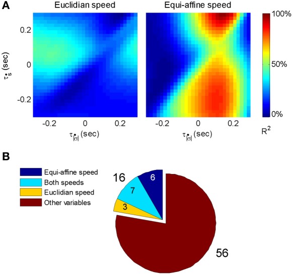
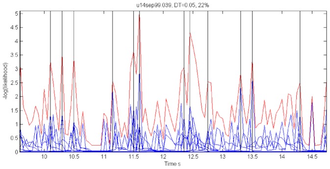
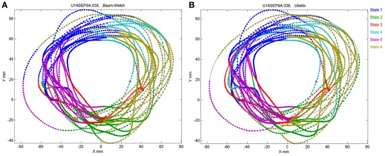
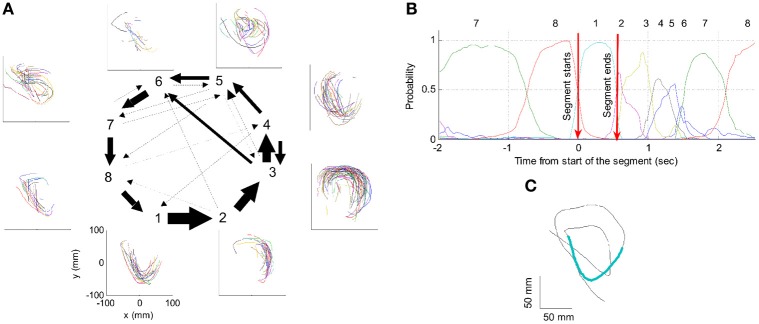
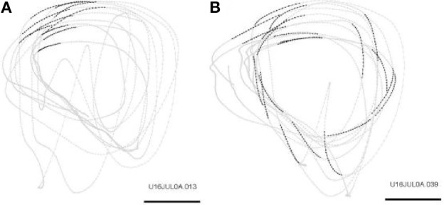
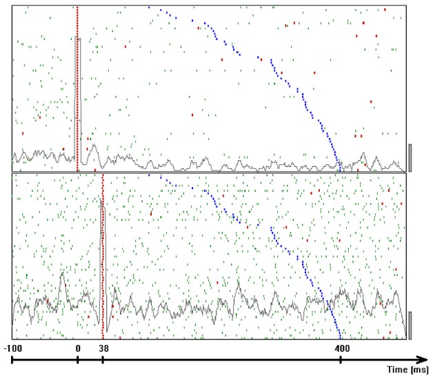
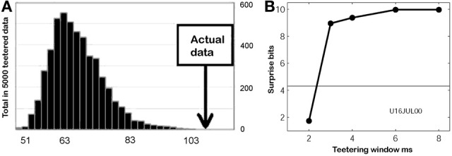
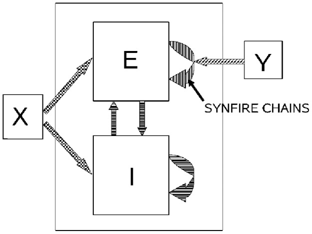
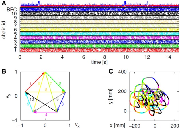
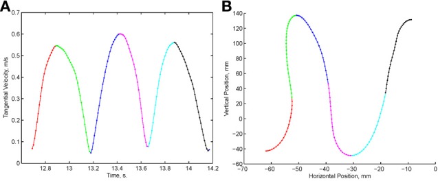
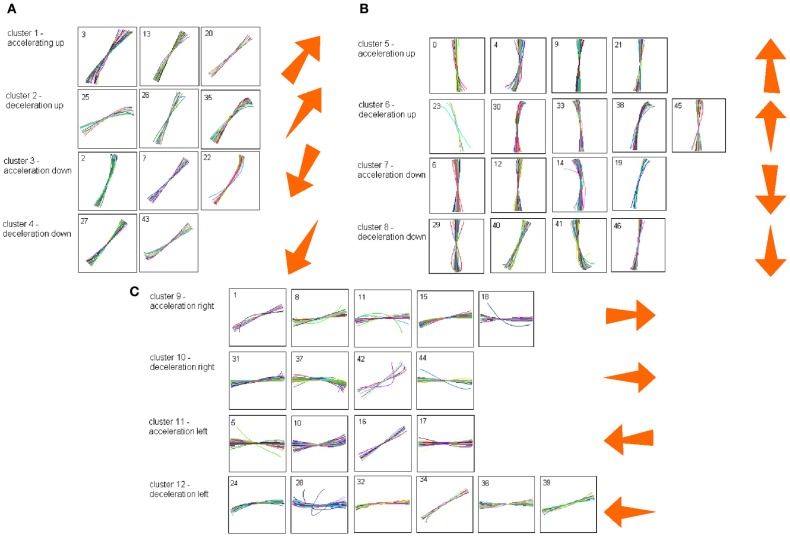
This article discusses the compositional structure of hand movements by analyzing and modeling neural and behavioral data obtained from experiments where a monkey (Macaca fascicularis) performed scribbling movements induced by a search task. Using geometrically based approaches to movement segmentation, it is shown that the hand trajectories are composed of elementary segments that are primarily parabolic in shape. The segments could be categorized into a small number of classes on the basis of decreasing intra-class variance over the course of training. A separate classification of the neural data employing a hidden Markov model showed a coincidence of the neural states with the behavioral categories. An additional analysis of both types of data by a data mining method provided evidence that the neural activity patterns underlying the behavioral primitives were formed by sets of specific and precise spike patterns. A geometric description of the movement trajectories, together with precise neural timing data indicates a compositional variant of a realistic synfire chain model. This model reproduces the typical shapes and temporal properties of the trajectories; hence the structure and composition of the primitives may reflect meaningful behavior.

Keywords: compositionality; hand-motion-model; motion-primitives; scribbling; synfire chains; voluntary-movements.

Figure 1

Parabolic elements of scribbling. (A) Sample drawing. Motion is sampled at 100/s (blue dots) points at which reward was given are marked by red circles. (B) Breaking a piece into 3 parabolas. Black dots—the measurements; red, green, magenta—three parabolas. (C) Changes over the course of training. For each parabolic segment two parameters were extracted: the orientation of the parabola and its focal distance. Those are plotted in the 2 dimensional (2-D) histogram. On the left is the histogram of the orientations (Y-marginal of the 2-D histogram). Each pair of histograms is for 1 training day. The left pair is for an early training session; the middle after a several months; and the right after half a year. Clearly, with training, three classes of parabolas emerged.

Figure 2

Parsing data to HMM states. Data for 41 s of scribbling is shown. Top bars give the sequence of hidden states as revealed by Viterbi training algorithm and Baum-Welch algorithm, respectively. The bottom graphs represent the probability of each possible state as a function of time (computed by the Baum–Welch algorithm). Most of the time there is only one dominant state and the transitions are steep. When no state had a probability above 0.5 the system was considered to be in an unknown state (left blank in the upper state bars).

Figure 3

HMM and drawings. The transition probabilities between states are coded by the thickness of the arrows. The actual drawing shapes associated with each HMM state are plotted near the state number. The different colors have no meaning, they are meant to facilitate discrimination among the various repetitions of similar shapes. State 1 appears to be associated with one parabola, while states 2 and 3 with the two others. The other states are associated with other drawings, many of which had to do with pausing or restarting to move.

Figure 4

Equi-affine differential geometry of monkey drawings. (A) Equi-affine velocity (dots) and curvature (+sign) for a scribbling segment. (B) The actual drawing made by the monkey. Since parabolas are characterized by zero equi-affine curvature, the motion segments can be well-fitted by parabolas (dashed lines).

Figure 5

Multi parameter tuning. Data for single units in motor cortex of a monkey tracing a convoluted trajectory. Three possible parameters were studied: position, velocity, and acceleration. For each of them all possible delays within ±250 ms were tried. The color within the cube shows the contribution to the variance of firing rate for one parameter (e.g., velocity) given the other two (e.g., position and acceleration). (A1) Velocity tuning. This single unit showed only one plane of higher contribution to the total variance. At the velocity cube (middle) we see a horizontal plane (for τ_vel) at time 70 ms (leading the velocity). (A2) Velocity and position tuning. For Position (given velocity and acceleration) we see a vertical plane at 0 delay and for the velocity (given position and acceleration) we see a horizontal plane leading the velocity by 90 ms. This single unit was coding two parameters at different delays.

Figure 6

Equi-affine tuning. As Euclidian velocity and equi-affine velocity have the same direction only the amplitude of the velocity vectors was considered here. All possible delay combinations within ±250 ms were evaluated. The (thick) vertical line when equi-affine speed was the main regressor indicates that this unit is tuned to equi-affine speed. The thickness of the line may be attributed to the fact that both types of speeds are highly correlated; hence the contribution of one, after factoring out the effect of the other, is noisy.${\tau }_{\left|\dot{\sigma }\right|}$ and τ_ṡ are the delays of the amplitudes of the equi-affine and Euclidian velocities.

Figure 7

Linear motion in velocity space. (A) Progression through groups of neuron positioned on a linear line in velocity space (black arrows). The polar coordinates (red arrows) of each group describe the direction and amplitude of the motion in Euclidian space. Each circle represents a large group of neurons with the same velocity tuning. (B) The shape of trajectory that the progressing activity will generate. Since the position of the groups is linear in the velocity space the produced motion is a parabola. If the speed of activity- progression is constant, then the drawing will obey the 2/3 power low. If instead of seven groups of neurons [as in (A)] we would have many more in between, the parabolas [in (B)] would be much smoother.

Figure 8

Simulations of the production of 3 parabolas. (A) The shape of the drawings generated by the simulation. (B) Raster plot of the activity in the network. Abscissa describes time, Ordinate provide the cell #. Activity of each neuron is described by dots along one line. The neurons along the ordinate are arranged according to their participation in the synfire chains. Synfire chains 4, 6, and 8 are the ones generating the drawing on the left. (C) The layout of the 3 synfire chains in velocity space. The synfire chain which is currently active is colored in thick red. At the moment activity is at the red dot producing the vertical motion near the maximal curvature of the parabola. Note that when one single synfire chain ends there is a competition among several others. E.g., at 750 synfire 6 ended and synfires 3, 7, and 8 show enhanced activity. After a short while synfire 8 wins.

Figure 9

Accuracy of spike intervals. Significance level for different teetering windows is shown for each experimental day whose significance was at least 2.5% for 10-ms precision. Abscissa is the teetering window (from 10 to 0.3 ms); ordinate is the probability value of finding the relation-score by chance. Because we looked for significant values in drawing components based on both direction and velocity separately, all probabilities have to be multiplied by 2. That is, a significance of 2.5% in this figure stands for a significance of 5%, and so forth. As can be seen, the days have significant values for teetering at 0.5, 2, 2, 3, 4, 6, and 8 ms.

Figure 10

Point of no return. (A) The drawing. (B) The tangential velocity. At the star the stop sound was given. The subject continued to draw for half a second producing two additional peaks of speed.

Figure 11

Sample of scribbling. Scribbling was sampled at 100/s. The subject scribbled until told to stop. Several such segments were concatenated for the analysis.

Figure 12

Conditional transition matrix.

Figure 13

Equi-affine analysis of drawing and parabolic fit. A short stretch of the monkey's drawing is shown. (A) Equi-affine analysis shows that between time 17.53 and 18.15 the equi-affine curvature (red) was almost 0. (B) Fit to parabolas was close to perfect. The section between 17.53 and 18.15 is between the green and red circles. It is fitted by two parabolas painted red and green.

Figure 14

Degree of fit and length of the parabolic strokes fitted to movement segments. (A) Euclidean lengths of the fitted parabolic strokes. In each plot, median values (over sessions) and 95% confidence intervals are shown. (B) Values of the D parameter estimating the error in fitting parabolas to the extracted segments.

Figure 15

Equi-affine curvature and its modifications with practice. (A) Distributions of equi-affine curvature (measured in mm^−4/3) for the first recording session, a session conducted following 16 practice days, and another session of well-trained behavior. (B) Distributions of the magnitude of the equi-affine curvature (same data).

Figure 16

Emerging parabolic clusters and dimensionality reduction. (A) Typical histograms for the fitted parabolic segments. In the one-dimensional histogram (left), the segments are counted according to their orientation. In the color histogram (right), they are counted in distinct bins according to the orientation and focal parameter of the parabola. (B) Location of the vertex and orientation of the parabola for every 10th parabolic segment for the recording sessions in (A). Locations of the vertices of the similarly oriented parabolas are also clustered. The clusters are marked by ellipses and the mean orientations of the parabolas within each cluster are depicted by arrows.

Figure 17

Motor cortical activity related to equi-affine speed. (A) Contribution matrices, used to compare the representation strength of Euclidean (left) and equi-affine (right) speeds in the activity of one motor cortical unit. Contributions are shown as fractions of the total (0.12 in this case) of a linear model including both speeds (see Equation 3). The vertical stripe in the right matrix indicates that the equi-affine speed is more strongly represented. The stripe appears at a time-lag of 0.12 s, where neural activity precedes the movement. This part was reproduced in Figure 6. (B) Number of movement-related units whose activities receive dominant contribution from the equi-affine and/or Euclidean speeds.

Figure 18

Cooperative changes in firing rates. Negative log-likelihood that the activity is stationary during a 5-s time interval. For all the spike trains we compute MLL_i = −log [prob(#spikes now | #spikes in the past 200 ms)] and MLL = ∑^M_{i = 1}MLL_i. We show the MLL of 11 well-isolated and stable spike trains (blue traces), the sum of the blue traces (red trace) and times of transition (black lines). Top 22% of the peaks were taken as transition times. Note that several individual MLL's have peaks at the same points indicating the tendency of cooperative changes in firing rates. For each such “stationary” piece we computed the mean firing rates of every single unit obtaining a vector of M firing rates. The vectors of mean firing rates were clustered into N groups by the k-means algorithm. The probability of transition from state i to state j was estimated by counting how many times activity assigned to group i was followed by activity assigned to group j. The firing rate for group i was computed by pulling together all the time slices judged to belong to group i. These were, then, used to initialize P and Λ.

Figure 19

Correspondence between drawing and HMM states. Data for 41 s of monkey's drawing is shown. Hand position was sampled at 100 Hz. Periods defined by the HMM state are plotted in different colors. For our data Baum–Welch (A) provided somewhat better fit with the drawings than the Viterbi training algorithm (B).

Figure 20

Illustration of movement segmentation according to a Hidden Markov Model (HMM). (A) An example of HMM results for one session. Center: Transition probabilities between states. The thickest arrows correspond to the highest probabilities, and the dashed and dotted arrows correspond to gradually lower probabilities. The largest depicted probability is about 15 times higher than the lowest depicted probability. Periphery: paths corresponding to the states (for presentation purposes, the paths with shortest and longest durations within each state were omitted so only 90% of the paths are shown). This part is reproduced in Figure 3. (B) Only a short time period of the data is illustrated. The HMM model, learned here for eight states, provides posterior probabilities as temporal functions. The neural activities can then be segmented based on the dominant probabilities. The numbers above the plot correspond to the state with the highest instantaneous probability. (C) The movement corresponding to the analysis in (B). The segment based on state 1 is highlighted; this segment is parabolic.

Figure 21

Drawing components. Examples of two drawing components during scribbling for 30 s. Scale bar is 50 mm. (A) Occurrences of the drawing component: “Transitions of drawing direction from a range of 180–210° to a range of 210–240°” are marked by larger dots. (B) Occurrences of the drawing component: “Transitions of drawing velocity from a range of 20–30 cm/s to a range of 10–20 cm/s” are marked by larger dots.

Figure 22

Frequent inter-spike intervals. Dot display showing occurrences of a frequent inter-spike interval around occurrences of the drawing component that was shown in Figure 21B. Top panel shows the firing times of unit 8.1. The bottom panel shows the firing times of unit 1.2. Each linelet represents a single spike. Linelets representing spikes which took part in the selected interval are colored red. The rasters were aligned on the first spike of the selected interval. The time of onset of the drawing is colored blue. Trials are sorted by increasing delays between the neural intervals and the drawing components. The gray line in each panel represents the average firing rate considering all 372 common occurrences using bins of 9 ms. Scale bars at the bottom right corner of each panel are 50 spikes per second.

Figure 23

Relations-score and teetered data. (A) Distribution of relations-scores for surrogate spike trains and the actual data. Five thousand surrogate spike trains were independently generated by teetering spike times within 10 ms. For each of these a relation-score was extracted. The distribution of these relations-score values was estimated by a histogram. The actual data had a value of 106.37 (arrow). None of the 5000 surrogate trains had a value above it. Hence the p-value for the actual data was estimated as less than 1/5000. (B) Surprise values for different teetering windows. Abscissa is the teetering window, ordinate is the surprise value. The horizontal line shows the surprise value for significance of 0.05. Thus, teetering within 3 ms already had a significant effect.

Figure 24

Sketch of the cortical network model. All connections between the 40,000 excitatory neurons in the model network are formed by synfire chains (vertically striped arrow). A neuron can occupy only one position in each chain but may contribute to several ones out of the total of 50 chains. Each chain consists of 20 pools each of which is fully connected to the next pool. The intra-chain synapses enable excitatory postsynaptic potentials (EPSPs) of a = 0.5 mV generated by alpha-function current with a rise time τα = 0.2. Synaptic delays are drawn from a uniform distribution between 0.5 and 3 ms, but are identical for all synapses connecting one pair of pools. Chains are stimulated at 1 Hz with independent Poisson sources. Stimuli arrive only at the neurons in the first pool of a chain and consist of 100 spike times drawn from a Gaussian distribution with standard deviation σ = 1 ms. In addition to the excitatory (E) neurons there are 10,000 inhibitory (I) neurons which are recurrently interconnected (horizontally striped arrows): each neuron establishes a random number of synapses drawn from a binomial distribution with the mean given by 10% of the size of the respective target population. EPSP amplitudes outside chains are a = 0.1 mV, inhibitory postsynaptic potential [IPSP] amplitude are 6-fold larger and have a rise time of 0.6 ms. Delay distributions are the same as within chains. Each neuron receives (cross-hatched arrows) an excitatory DC drive of 350 pA. Further parameters for the integrate-and-fire point neurons are τ = 20 ms, C = 250 pF, θ = 20 mV, τref = 2 ms. Excitatory neurons are randomly chosen to form 50 completely connected synfire chains (vertically striped arrow). A neuron can occupy only one position in each chain but may contribute to several chains. Intra-chain synapses are 5-fold stronger than other EPSPs. Intra-chain delays are drawn from the same distribution as others but are identical for synapses connecting a particular pair of neuron links. Chains are stimulated at 1 Hz with independent Poisson sources. A stimulus consists of 100 spike times drawn from a Gaussian distribution with standard deviation σ = 1 ms and is received by all the neurons of the first link in a chain.

Figure 25

Raster representation of the activity of the neurons in a particular synfire chain. (A) The randomly assigned neuron numbers have been remapped so that the 2000 neurons of the chain are labeled 8001–10,000 (ordinate). The data show an arbitrary 10-s segment (abscissa) of activity. The thin black, almost vertical lines represent runs of this chain. (B) Temporal magnification of a portion of (A). Two complete runs and one partial run of the chain are shown. At this timescale the nearly synchronous activity of each link in the chain becomes visible, as does the propagation time between links.

Figure 26

Fluctuations in network activity. (A) Raster of 150 randomly selected neurons (ordinate) during a period of 5 s (abscissa). The activity of the neurons appears uncorrelated, irregular, and fairly stationary in time. (B) A raster of 10,000 neurons during the same time period as in (A). The activity exhibits prominent vertical bands.

Figure 27

Relation of population firing rate and synfire activation rate. The black curve represents the smoothed population activity (triangular filter, full width 51 ms); the gray curve represents smoothed stimulation times (same filter) of all synfire chains. The actual stimulation times are shown as vertical bars at the bottom.

Figure 28

Mapping synfire activity to parabolic movements. (A) The preferred velocity vectors for the pools of the synfire chain (gray arrows; shown for every third pool of the chain) are determined by sampling a straight line in velocity space (red arrow). (B) The spiking activity of an activity volley propagating with constant speed along a synfire chain. Preferred velocity vectors for every third pool as in (A) are shown as gray arrows above the dot display. (C) Generated parabolic trajectory. The black cross at (0,0) indicates the start position.

Figure 29

Generation of scribbling trajectories. (A) Spiking activity of bidirectional and synfire chain networks. Colors of the activity of each chain corresponds to the colors of the arrow in velocity space shown in (B). Above the raster plot the average firing rate of the synfire network (red) and the bidirectional network (blue) is plotted. (B) Abstract generator for trajectories consisting of parabolic segments. Uniform motion along straight lines in velocity space is equivalent to parabolic motion in position space. Each colored arrow represents a parabolic segment and its direction of execution. When the end of an arrow is reached, one of the two successor arrows is selected. (C) Scribbling trajectory extracted from the spiking activity using population coding. Segments are drawn in the color of the most active synfire chain.

Figure 30

Breaking a drawing into strokelets. One second of human drawing is shown. (A) The tangential velocity. (B) The drawing. Each strokelet is colored differently to facilitate visualization.

Figure 31

Clustering of strokelets. Each little panel shows all the strokelets that belong to one group. They are colored differently to facilitate visual discrimination among them. All the strokelets within the same group are stretched to the same length and plotted on top of each other. Each line of groups belongs to the same cluster. The arrow to the right of each row represents the direction of motion in this cluster. Expanding arrows symbolize accelerating strokelets and shrinking arrow represent decelerating ones. (A) oblique movements. (B) Vertical movements. (C) horizontal movements.

References

1. Abeles M. (1982). Local Cortical Circuits: an Electrophysiological Study. Berlin; New York: Springer-Verlag
1. Abeles M. (1991). Corticonics: Neural Circuits of the Cerebral Cortex. New York, NY: Cambridge University Press; 10.1017/CBO9780511574566 - DOI
1. Abeles M., Bergman H., Gat I., Meilijson I., Seidemann E., Tishby N., et al. (1995). Cortical activity flips among quasi-stationary states. Proc. Natl. Acad. Sci. U.S.A. 92, 8616–8620 10.1073/pnas.92.19.8616 - DOI - PMC - PubMed
1. Abeles M., Goldstein M. H. (1977). Multispike train analysis. Proc. IEEE 65, 762–773 10.1109/PROC.1977.10559 - DOI
1. Amarasingham A., Hastopoulos N., Geman S. (2003). At what time scale does the nervous system operate? Neurocomputing 52, 25–29
LinkOut - more resources