

From birdsong to human speech recognition: bayesian inference on a hierarchy of nonlinear dynamical systems
- PMID: 24068902
- PMCID: PMC3772045
- DOI: 10.1371/journal.pcbi.1003219
From birdsong to human speech recognition: bayesian inference on a hierarchy of nonlinear dynamical systems
Abstract
Our knowledge about the computational mechanisms underlying human learning and recognition of sound sequences, especially speech, is still very limited. One difficulty in deciphering the exact means by which humans recognize speech is that there are scarce experimental findings at a neuronal, microscopic level. Here, we show that our neuronal-computational understanding of speech learning and recognition may be vastly improved by looking at an animal model, i.e., the songbird, which faces the same challenge as humans: to learn and decode complex auditory input, in an online fashion. Motivated by striking similarities between the human and songbird neural recognition systems at the macroscopic level, we assumed that the human brain uses the same computational principles at a microscopic level and translated a birdsong model into a novel human sound learning and recognition model with an emphasis on speech. We show that the resulting Bayesian model with a hierarchy of nonlinear dynamical systems can learn speech samples such as words rapidly and recognize them robustly, even in adverse conditions. In addition, we show that recognition can be performed even when words are spoken by different speakers and with different accents-an everyday situation in which current state-of-the-art speech recognition models often fail. The model can also be used to qualitatively explain behavioral data on human speech learning and derive predictions for future experiments.
Conflict of interest statement
The authors have declared that no competing interests exist.
Figures
 and
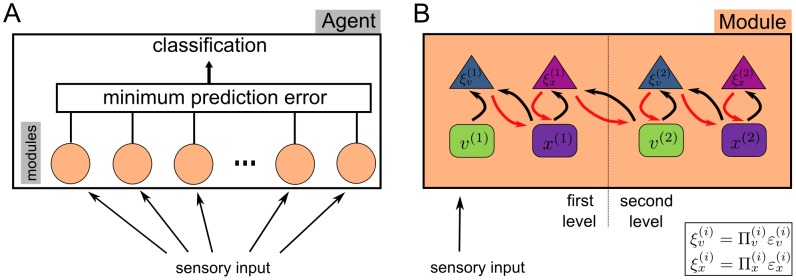
and  , respectively) try to minimize the precision-weighted prediction errors (
 and
and  ) by exchanging messages. Predictions are transferred from second level to the first and prediction error is propagated back from the first to the second level (see section Model: Learning and Recognition for more details). Adapted from .
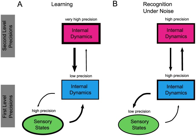
 and internal log-precision:
  where
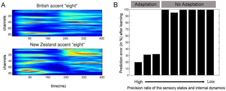
where  from left to right). For each precision ratio, we plotted the reduction in prediction error (of the causal states, see Model) after five repetitions of the word “eight” spoken with a New Zealand accent. As expected, accent adaptation was accomplished only with high sensory/internal precision ratios (resulting in greatly reduced prediction errors) whereas no adaptation occurred (prediction errors remained high) when this ratio was low.
References
-
- Bolhuis JJ, Okanoya K, Scharff C (2010) Twitter evolution: converging mechanisms in birdsong and human speech. Nature Reviews Neuroscience 11: 747–759. - PubMed
-
- Doupe AJ, Kuhl PK (1999) Birdsong and human speech: Common themes and mechanisms. Annual Review of Neuroscience 22: 567–631. - PubMed
-
- Creutzfeldt O, Ojemann G, Lettich E (1989) Neuronal-Activity in the Human Lateral Temporal-Lobe .1. Responses to Speech. Experimental Brain Research 77: 451–475. - PubMed
-
- Berwick RC, Okanoya K, Beckers GJL, Bolhuis JJ (2011) Songs to syntax: the linguistics of birdsong. Trends in Cognitive Sciences 15: 113–121. - PubMed
Publication types
MeSH terms
LinkOut - more resources
Full Text Sources
Other Literature Sources
