Stochastic calcium mechanisms cause dendritic calcium spike variability

Abstract

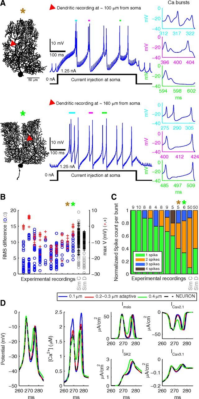
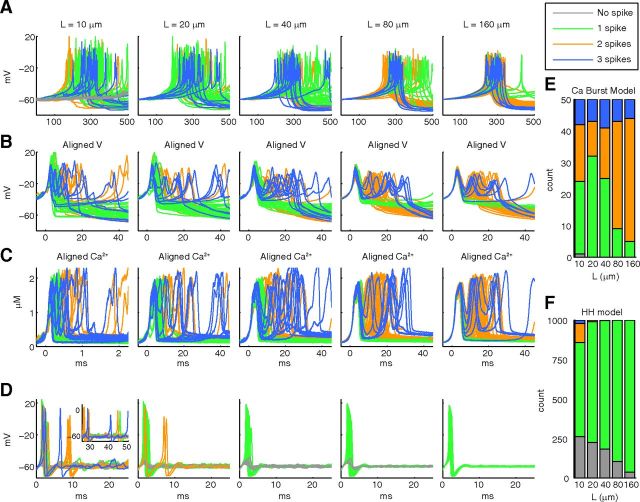
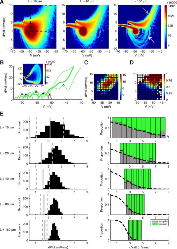
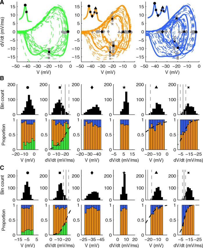
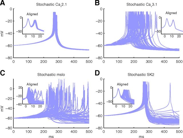
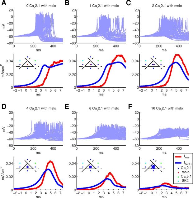
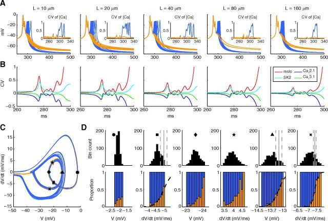
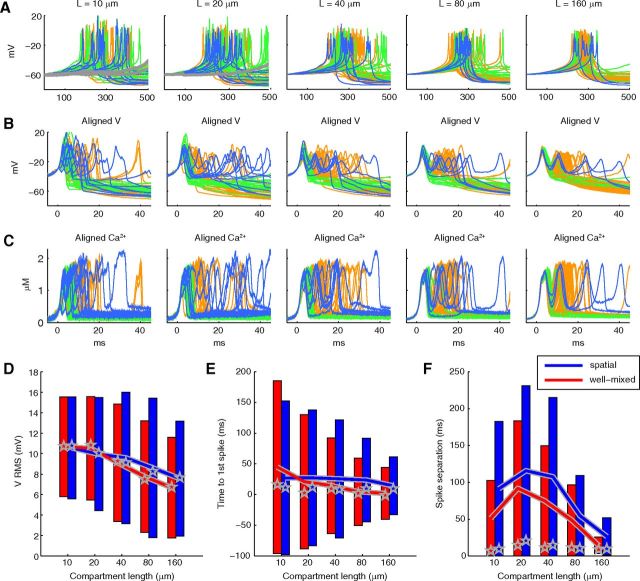
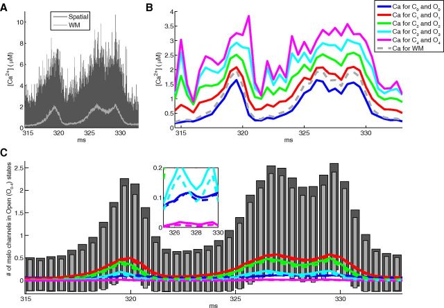
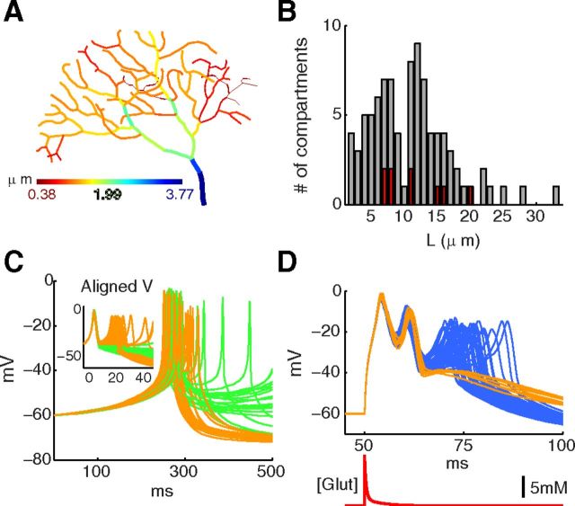
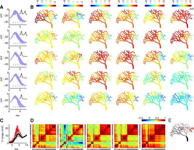
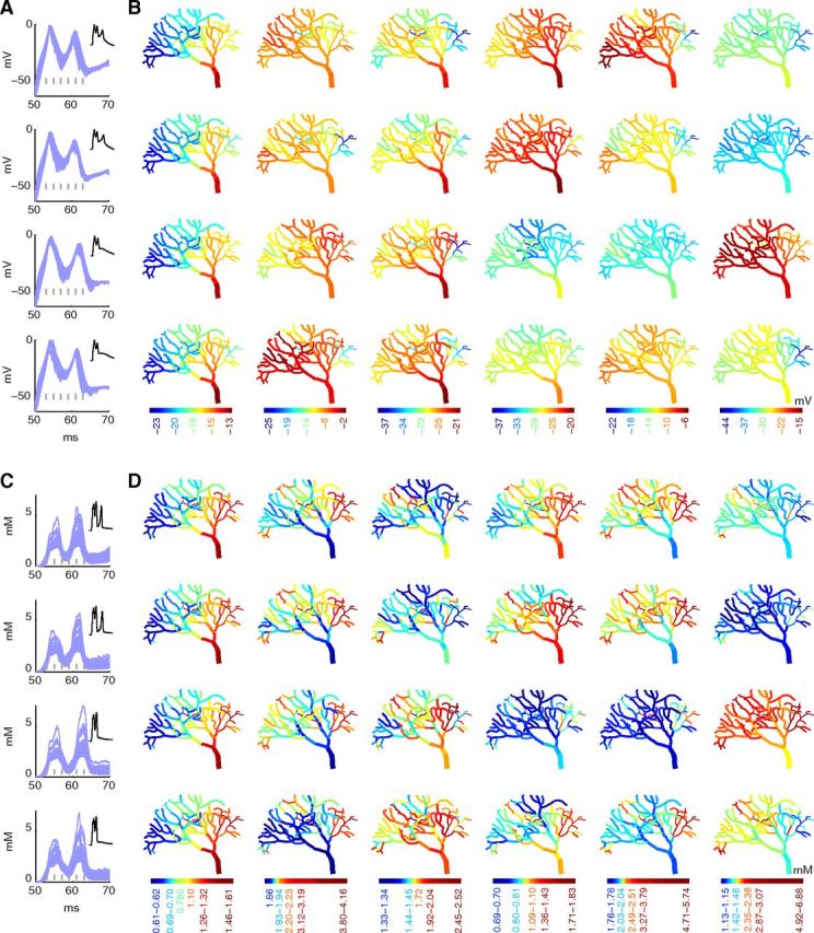
Bursts of dendritic calcium spikes play an important role in excitability and synaptic plasticity in many types of neurons. In single Purkinje cells, spontaneous and synaptically evoked dendritic calcium bursts come in a variety of shapes with a variable number of spikes. The mechanisms causing this variability have never been investigated thoroughly. In this study, a detailed computational model using novel simulation routines is applied to identify the roles that stochastic ion channels, spatial arrangements of ion channels, and stochastic intracellular calcium have toward producing calcium burst variability. Consistent with experimental recordings from rats, strong variability in the burst shape is observed in simulations. This variability persists in large model sizes in contrast to models containing only voltage-gated channels, where variability reduces quickly with increase of system size. Phase plane analysis of Hodgkin-Huxley spikes and of calcium bursts identifies fluctuation in phase space around probabilistic phase boundaries as the mechanism determining the dependence of variability on model size. Stochastic calcium dynamics are the main cause of calcium burst fluctuations, specifically the calcium activation of mslo/BK-type and SK2 channels. Local variability of calcium concentration has a significant effect at larger model sizes. Simulations of both spontaneous and synaptically evoked calcium bursts in a reconstructed dendrite show, in addition, strong spatial and temporal variability of voltage and calcium, depending on morphological properties of the dendrite. Our findings suggest that stochastic intracellular calcium mechanisms play a crucial role in dendritic calcium spike generation and are therefore an essential consideration in studies of neuronal excitability and plasticity.

Figure 1.

Experimentally recorded dendritic calcium spikes show large variability. A, Example electrophysiological traces recorded from the dendrite of two PCs (shown on left). The bursts of dendritic Ca²⁺ spikes were recorded from the dendrite (recording location is marked with red triangles) while injecting 1.25 nA current at the soma. For both cells, three of the bursts of Ca²⁺ spikes (see Materials and Methods) are enlarged and displayed in cyan, purple, and green insets to show the variability in number of spikes (1–3 spikes per burst), variability in duration of burst (10–40 ms), and variability in spike amplitudes, respectively. The small spikelets in the traces both before and during the current injection are passively propagated somatic action potentials. B, C, Data recorded from 10 different PCs show robust variability of dendritic calcium bursts. B, The circles represent RMS differences (ordinate axis on left hand side) between every pair of bursts of Ca²⁺ spikes in recordings and for the spatial (Sim C) and dendrite (Sim D) models (Figs. 2A, 160 μm; and 10C, respectively). +, Maximum voltage level of every spike (ordinate axis on right hand side) in each recording and for the spatial (Sim C) and dendrite (Sim D) models. C, Variability of spikes count per burst of Ca²⁺ spikes in recordings and for the spatial (Sim C) and dendrite (Sim D) models. Number of bursts detected in each trace are marked at the top of each bar. B, C, Cells marked with brown and green asterisks are shown in A. Data provided by Ede Rancz and Michael Häusser (University College London; see Materials and Methods). D, Three different tetrahedral meshes describing the same cylindrical compartment of length 1 μm and diameter 2 μm are used for spatial deterministic simulations in STEPS and compared with the NEURON benchmark. The 0.2–0.3 μm adaptive mesh was found to give an almost perfect match to the benchmark. Panels show, from left to right, membrane potential, submembrane calcium concentration, and current density for the four different ion channels.

Figure 2.

The stochasticity of a calcium burst model persists with increase in model size, whereas that of a sodium spike model decreases with model size. A, Nonaligned voltage traces (50 iterations for each model size) obtained from simulations of the detailed calcium burst model with stochastic ion channels and stochastic intracellular Ca²⁺ dynamics and 3D diffusion for various length cylindrical meshes. The voltage traces plotted in gray, green, orange, and blue represent traces with no spike, 1 spike, 2 spikes, and >2 spikes, respectively. B, Same data, aligned at −30 mV in 50 ms windows. C, The corresponding calcium traces, aligned at threshold of −30 mV in the voltage traces. D, Spontaneously generated sodium spikes (50 iterations for each model size) using a stochastic HH model in the same meshes. Inset (in panel for 10 μm length), Later part of the respective traces. E, Histogram of number of voltage traces (iterations) with no spike, 1 spike, 2 spikes, and >2 spikes for different length compartments for the calcium burst model shows that variability in burst characteristics persist for large model sizes. F, A similar histogram for the sodium spike model (1000 iterations for each model size) shows a more rapid decrease in variability with increase in model size.

Figure 3.

Phase space analysis of HH model explains variability dependence on model size. For phase space analysis, the raw voltage signals were smoothed by convolution with a Hanning window on interval −0.1 ms to 0.1 ms. A, Phase space heat maps of 1000 trials of the HH model are shown for the 10, 40, and 160 μm meshes, showing the spontaneous fluctuations around the baseline and the spike-initiation region. Right, Gray arrow indicates a successful spike. White arrow indicates a failed spike. B, Top, Full phase space heat map of the HH model at 10 μm (expanded from A) showing both initial and spontaneous spikes. Boxed region is shown in more detail in bottom. Bottom, dV/dt peaks of fluctuations are detected for 3 cases that resulted in a spontaneous spike (green, peaks marked by circles) and 3 cases with no spike (gray, peaks marked by triangles). Spontaneous spikes tend to originate from larger dV/dt peaks that occur at higher voltages (circles) compared with peaks that did not result in a spike (triangles), although there is some crossover. C, D, All spontaneous spikes from 5000 trials of the 10 μm model are shown as (C) position by peak dV/dt and V at which each spike originated (color bar scale is number of spikes per bin) and (D) for each phase space bin the probability of a peak resulting in a spontaneous spike (computed as the proportion of dV/dt peaks that resulted in a spontaneous spike divided by those that did not). These panels match the region denoted by a square in A (left). E, Left, For 1000 trials at each mesh length, the distribution in dV/dt at which voltage of −60 mV was first crossed. Right, For these distributions, the proportion of trials by dV/dt position that resulted in a spike (green) or spike failure (gray). Sigmoidal curves were fitted by weighted least-squares fit to define a sigmoidal separatrix. The point at which the value of the sigmoidal is 0.5 is illustrated in the left panels (solid gray line) as the approximate location of a probabilistic phase boundary. Dashed gray lines indicate the points at which the value of the fitted sigmoidal is 0.3 and 0.7.

Figure 4.

Phase space analysis of stochastic calcium burst model shows wide probabilistic phase boundaries. A total of 500 trials each for the 80 and 160 μm meshes are analyzed. The raw voltage signals were smoothed by convolution with a Hanning window on interval −0.5 ms to 0.5 ms. A, Ten example phase plots from the 160 μm compartment each for 1 spike (green), 2 spike (orange), and 3 spike (blue) trials. Full line indicates one phase plot (voltage trace shown in inset); the other nine are shown as broken lines for clarity. Symbols show six phase positions analyzed further in B and C: circle represents the voltage peak of the first spike (dV/dt = 0); square represents the fall after the first spike to −20 mV; diamond represents the voltage minimum between first and second spike (dV/dt = 0); star represents the rise to second spike at −20 mV; triangle represents the voltage peak of the second spike (dV/dt = 0); cross represents the fall after the second spike to −23 mV. B, C, Histograms represent distribution of all trials as number of trials (top), and proportion of trials that resulted in 1 spike (green), 2 spikes (orange), or 3 spikes (blue) (bottom) for 80 μm (B) and 160 μm (C). The abscissa used (V or dV/dt) depends on the phase position analyzed. For the positions denoted by square, triangle, and cross, sigmoidal curves were fitted by weighted least-squares fit to define a sigmoidal separatrix. The point at which the value of the sigmoidal is 0.5 is illustrated in the top panels (solid gray line, for the triangle in B the boundary falls outside the figure), and the points at which the value of the fitted sigmoidal is 0.3 and 0.7 are shown as dashed gray lines.

Figure 5.

The stochastic effect of Ca²⁺-activated K⁺ channels is large compared with the stochastic effect of voltage-gated Ca²⁺ channels. A–D, Voltage traces for 50 iterations are plotted using a hybrid model (with compartment length of 10 μm) with (A) stochastic Ca_v2.1 channels, (B) stochastic Ca_v3.1 channels, (C) stochastic mslo channels, and (D) stochastic SK2 channels. All other mechanisms, except the mentioned stochastic channels, are simulated deterministically. A–D, Insets, Aligned traces at −30 mV to highlight the variability of spike features in each model over multiple runs.

Figure 6.

The clustering of Ca_v2.1 channels with mslo channels has a strong effect on dendritic excitability. A–F, Simulations of the stochastic calcium burst model with a variable number of Ca_v2.1 channels clustered together with each mslo channel, sharing the membrane space and submembrane volume. A cylinder of 2 μm diameter and 40 μm length was simulated, and the total number of ion channels were constant for all simulations. Top, Voltage traces for 50 iterations (not aligned). Bottom, Spike-triggered average traces of the Ca_v2.1 and mslo currents. Inset, Schematic of how channels were arranged in the surface triangles of the mesh.

Figure 7.

The stochastic effect of Ca²⁺ dynamics is sustained at large model size. A, The voltage traces (50 iterations for each model size) obtained from simulations of the detailed calcium spike model with deterministic ion channels and stochastic Ca²⁺ dynamics for meshes of varying length. Top insets, CV of resulting intracellular calcium concentration during the burst. The voltage traces and CV are color coded for bursts with 2 spikes (orange) or 3 spikes (blue). B, The corresponding CV of ionic currents during a 40 ms time window covering the calcium burst. A decreasing CV for all currents during the first and second spike with increasing compartment length can be observed. C, D, Phase analysis for the 40 μm compartment at the following: circle represents the peak of the first spike (dV/dt = 0); square represents the fall after the first spike to −20 mV; diamond represents the minimum between first and second spike (dV/dt = 0); star represents the rise to second spike at −20 mV; triangle represents the peak of the second spike (dV/dt = 0); cross represents the fall after the second spike to −23 mV. C, D, Organized similarly to Figure 4A, B, respectively.

Figure 8.

Detailed calcium burst model simulated under well-mixed stochastic conditions captures important features of variability. A, Nonaligned voltage traces (50 iterations for each model size) for the well-mixed stochastic model for various length compartments. The voltage traces plotted in gray, green, orange, and blue represent traces with no spike, 1 spike, 2 spikes, and >2 spikes, respectively. B, Same data, aligned at −30 mV in 50 ms windows. C, The corresponding calcium traces, aligned at threshold of −30 mV in the voltage traces. D–F, Analysis of variability for different model sizes for the spatial model (data from Fig. 2) and the well-mixed model (this figure). All measures are taken relative to the deterministic solution and expressed as the tolerance interval for 90% of the data at 90% confidence for the proper distribution. Lines connect the midpoints. Stars indicate the median. D, RMS of voltage (normal distribution). E, Timing of first spike (γ distribution). F, Time separation between first and second spike if second spike present (γ distribution).

Figure 9.

Local calcium concentrations give greater overall mslo activation and larger variability compared with well-mixed conditions. A, Calcium recordings from a stochastic calcium burst simulation at 10 μm, for each of 127 intracellular tetrahedrons connected to a triangle containing an mslo channel. The concentration range across all tetrahedrons is shown at each time point (dark gray) along with the concentration that would be sampled by each channel under well-mixed conditions (light gray). Two simulations mimicking spatial and well-mixed activation of the mslo channel were simulated 10,000 times. B, In the spatial simulation, the observed mean calcium concentration per activated mslo channel shows a dependence on state, with each progressively higher activation state showing a greater mean calcium concentration. C, Mean open state populations across trials for spatial simulations (colored lines) and well-mixed simulations (colored dashes) are compared showing marginally, yet consistently, higher activation in spatial simulations for every state. Total activation is shown as mean ± SD across trials for spatial (dark gray) and well-mixed (light gray) simulations, showing a small yet consistently larger variation in activation for the spatial simulations.

Figure 10.

The stochastic effect of calcium-related mechanisms persists in dendritic morphologies. A, The PC dendrite morphology with 100 compartments used to simulate both spontaneous and synaptically evoked stochastic calcium bursts. The compartments are color-coded according to their diameters. Total length and total surface area of the dendritic tree is 1098 μm and 5716.6 μm², respectively. B, A histogram of lengths of dendritic compartments shows that the distribution of dendrites with small diameters (in red; diameter <0.7 μm as marked in red in Fig. 11) is spread uniformly across the distribution of dendrites with large diameters (in gray; diameter ≥0.7 μm as color coded in different shades of gray in Fig. 11). C, Voltage traces of spontaneous calcium bursts recorded from the first dendritic compartment over 50 trials. The voltage traces shown are classified into bursts with 1 spike (green) and bursts with 2 spikes (orange). Inset, Same data aligned at −30 mV. A second spontaneous burst sometimes occurs. D, Voltage traces of synaptically evoked calcium bursts recorded from the first dendritic compartment of the morphology over 50 trials. The voltage traces are classified into bursts with 2 spikes (orange) and bursts with 3 spikes (blue). The red trace shown below is the glutamate pulse applied to activate AMPA receptors in primary dendrite compartments (blue in A).

Figure 11.

Stochastic calcium bursts in a dendrite model show large spatiotemporal variation of membrane potentials. This figure shows voltage during five different runs of the stochastic well-mixed model of a PC dendrite (A–E). A, B, In the first two runs, the burst consisted of 2 calcium spikes; in the other runs, only 1 calcium spike was generated. A, First 8 ms of the voltage traces recorded from all compartments of the dendritic tree are overlaid. Inset, Complete burst. Gray vertical lines indicate the time points for which the spatial maps are shown. B, Spatial maps of membrane potential throughout the dendrite for each time point marked with gray lines in A. Each time point has its own linear color scale to emphasize differences within single maps. C, Voltage range for all compartments (difference of maximum V and minimum V at each time point across 50 trials). Gray represents compartments with diameter ≥0.7 μm; red represents smaller-diameter ones; black represents mean. D, Spatial correlation of voltage of first 5 time points across 50 trials. Different shades of gray are used in sidebars to highlight subtrees as shown in E. Dendrites with diameter <0.7 μm are marked with red dots. E, Dendritic tree plotted in different shades of gray to highlight two subtrees stemming out of the primary dendritic branch plotted in black. Red circles represent dendrites with diameter <0.7 μm.

Figure 12.

Stochastic synaptically evoked calcium burst model generates differential patterns of voltage and calcium across dendrite. This figure shows voltage and calcium during four different runs of the synaptically evoked dendritic calcium burst model (A–D). A, B, In the first two runs, the burst consisted of 3 calcium spikes; in the other runs, only 2 calcium spikes were generated. A, First 20 ms of the voltage traces recorded from all compartments of the dendritic tree are overlaid. Inset, Complete burst. Gray vertical lines indicate the time points for which the spatial maps are shown. B, Spatial maps of membrane potential throughout the dendrite for each time point marked with gray lines in A. Each time point has its own linear color scale to emphasize differences within single maps. C, D, Calcium traces for calcium bursts shown in A. C, Calcium traces corresponding to the voltage traces recorded from all compartments of the dendritic tree are overlaid. Inset, Complete calcium transient. Gray vertical lines indicate the time points for which the spatial maps are shown. D, Spatial maps of submembrane calcium concentration throughout the dendrite for each time point marked with gray lines in C. Each time point has its own color scale to emphasize differences within single maps. The color scales used in these maps are nonlinear (using histogram equalization) to enhance the contrast.

References

1. Antunes G, De Schutter E. A stochastic signaling network mediates the probabilistic induction of cerebellar long-term depression. J Neurosci. 2012;32:9288–9300. doi: 10.1523/JNEUROSCI.5976-11.2012. - DOI - PMC - PubMed
1. Anwar H, Hong S, De Schutter E. Controlling Ca(2+)-activated K (+) channels with models of Ca (2+) buffering in Purkinje cells. Cerebellum. 2012;11:681–693. doi: 10.1007/s12311-010-0224-3. - DOI - PMC - PubMed
1. Belmeguenai A, Hosy E, Bengtsson F, Pedroarena CM, Piochon C, Teuling E, He Q, Ohtsuki G, De Jeu MT, Elgersma Y, De Zeeuw CI, Jörntell H, Hansel C. Intrinsic plasticity complements long-term potentiation in parallel fiber input gain control in cerebellar Purkinje cells. J Neurosci. 2010;30:13630–13643. doi: 10.1523/JNEUROSCI.3226-10.2010. - DOI - PMC - PubMed
1. Berkefeld H, Fakler B, Schulte U. Ca2+-activated K+ channels: from protein complexes to function. Physiol Rev. 2010;90:1437–1459. doi: 10.1152/physrev.00049.2009. - DOI - PubMed
1. Bittner KC, Hanck DA. The relationship between single-channel and whole-cell conductance in the T-type Ca2+ channel Ca(V)3.1. Biophys J. 2008;95:931–941. doi: 10.1529/biophysj.107.128124. - DOI - PMC - PubMed
Publication types
LinkOut - more resources