Transmembrane current imaging in the heart during pacing and fibrillation

Abstract

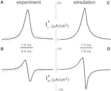
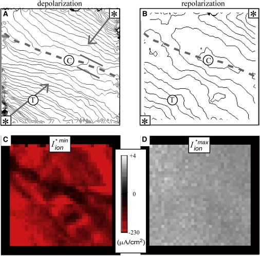
Recently, we described a method to quantify the time course of total transmembrane current (Im) and the relative role of its two components, a capacitive current (Ic) and a resistive current (Iion), corresponding to the cardiac action potential during stable propagation. That approach involved recording high-fidelity (200 kHz) transmembrane potential (Vm) signals with glass microelectrodes at one site using a spatiotemporal coordinate transformation via measured conduction velocity. Here we extend our method to compute these transmembrane currents during stable and unstable propagation from fluorescence signals of Vm at thousands of sites (3 kHz), thereby introducing transmembrane current imaging. In contrast to commonly used linear Laplacians of extracellular potential (Ve) to compute Im, we utilized nonlinear image processing to compute the required second spatial derivatives of Vm. We quantified the dynamic spatial patterns of current density of Im and Iion for both depolarization and repolarization during pacing (including nonplanar patterns) by calibrating data with the microelectrode signals. Compared to planar propagation, we found that the magnitude of Iion was significantly reduced at sites of wave collision during depolarization but not repolarization. Finally, we present uncalibrated dynamic patterns of Im during ventricular fibrillation and show that Im at singularity sites was monophasic and positive with a significant nonzero charge (Im integrated over 10 ms) in contrast with nonsingularity sites. Our approach should greatly enhance the understanding of the relative roles of functional (e.g., rate-dependent membrane dynamics and propagation patterns) and static spatial heterogeneities (e.g., spatial differences in tissue resistance) via recordings during normal and compromised propagation, including arrhythmias.

Figure 1

Schematic illustrating the measurement of V_i, V_e, and fluorescent transmembrane potential F_m from the surface of the isolated rabbit heart. The steps required for computing ion-current images involve the calibration (indicated by asterisks) of F_m, I_m, I_c, and I_ion. (RA, right atrium; LA, left atrium; RV, right ventricle; LV, left ventricle; CCD, charge-coupled device fluorescent-imaging camera; x, horizontal; y, vertical image axes of CCD; t, time; AR, anisotropy ratio; ϕ, fiber angle.) Other abbreviations are defined in Table 1. I_m is computed as the second spatial derivative of F_m using a nonlinear local surface fit (polyfit); the details of the methodology shown here are provided in the text (see Methods; see Algorithm Development).

Figure 2

Calibration of transmembrane currents computed from fluorescence transmembrane signals in experiments (F^∗_m) and simulations (V_opt). (A) I_c computed from microelectrode data (thick line) and I^∗_c computed from F^∗_m at a nearby site and scaled (thin line). (B) I_m computed from microelectrode data (thick line) and I^∗_m computed from the spatial gradient of F^∗_m at a site closest to the microelectrode and scaled (thin line). (C) I_c computed from simulated V_m (thick line) and I^∗_c computed from V_opt at a the same site and scaled (thin line). (D) I_m computed from simulated V_m (thick line) and I^∗_m computed from the spatial gradient of V_opt and scaled (thin line). Details of this calibration are provided in Algorithm Development.

Figure 3

Transmembrane current imaging during wave collision resulting from pacing at two sites (locations indicated by asterisks in the lower-left and upper-right corners). (A) Isochrone map indicating the position of the wave front at 1-ms intervals. (Gray solid lines) Direction of propagation. (Dashed gray lines) Intersection of two waves. (Parallel gray lines) Collision and block. (B) Time course of transmembrane potential as recorded using a fluorescence probe (F^∗_m) in the upper-left panel and calibrated transmembrane current density (I^∗_ion, black; I^∗_m, red; I^∗_c, blue) signals at the five labeled locations during depolarization. (C) Snapshots of F^∗_m, I^∗_m, and I^∗_ion at two instants of time (indicated by the two vertical dashed lines in the F_m plot in panel B).

Figure 4

Analysis of I^∗_ion spatial distribution during a wave collision. (A) Isochrone map indicating the position of the wave front (depolarization) at 1-ms intervals. (B) Isochrone map indicating the position of the wave tail (repolarization) at 5-ms intervals. (C) Spatial distribution of I^∗min_ion that occurs during depolarization. (D) Spatial distribution of I^∗max_ion that occurs during repolarization. Note the different timescale of isochrones and magnitude of I^∗_ion for depolarization and repolarization.

Figure 5

Transmembrane current imaging of focal activation and wave collision during fibrillation (noncalibrated I_m values only). (A) Isochrone map indicating the position of the wave front at 1-ms intervals demonstrating focal activation from two locations followed by collision. Time course of transmembrane potential (B) as recorded using a fluorescence probe (F^∗_m) at two sites (C) and the corresponding I^F_m signals. (D) Snapshots of F^∗_m, I^F_m, and θ at two instants of time (indicated by vertical dashed lines in panels B and C). The value θ was computed at each site as $\arctan \left[F_m^{\ast }\left(t+\tau \right)-F_{50},F_m^{\ast }\left(t\right)-F_{50}\right]$, where F₅₀ represents 50% of F^∗_m range and τ = 10 ms.

Figure 6

Transmembrane current imaging of reentry during fibrillation (relative I_m values only). (A) Isochrone map indicating the position of the wave front at 1-ms intervals demonstrating reentry. Time course of transmembrane potential (B) F^∗_m at two sites and the corresponding I^F_m (C) signals. (D) Snapshots of F^∗_m, I^F_m, and θ at two instants of time (indicated by vertical dashed lines in panels B and C). Phase singularity sites are indicated in θ images as minus signs, indicating counterclockwise rotation.

Figure 7

Comparison of membrane current I^F_m (A) and membrane charge Q^F_m (B) at phase singularity sites (grey) and nonphase-singularity sites (black). The value n refers to values computed from every 10-ms interval at each location.

References

1. Cabo C., Pertsov A.M., Jalife J. Wave-front curvature as a cause of slow conduction and block in isolated cardiac muscle. Circ. Res. 1994;75:1014–1028. - PubMed
1. Gray R.A., Jalife J., Pertsov A.M. Nonstationary vortexlike reentrant activity as a mechanism of polymorphic ventricular tachycardia in the isolated rabbit heart. Circulation. 1995;91:2454–2469. - PubMed
1. Wikswo J.P., Jr., Lin S.F., Abbas R.A. Virtual electrodes in cardiac tissue: a common mechanism for anodal and cathodal stimulation. Biophys. J. 1995;69:2195–2210. - PMC - PubMed
1. Gray R.A., Jalife J., Pertsov A.M. Mechanisms of cardiac fibrillation. Science. 1995;270:1222–1223. - PubMed
1. Gray R.A., Pertsov A.M., Jalife J. Spatial and temporal organization during cardiac fibrillation. Nature. 1998;392:75–78. - PubMed
Publication types
LinkOut - more resources