A single-molecule long-read survey of the human transcriptome

Abstract

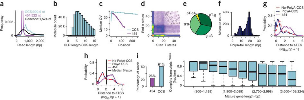
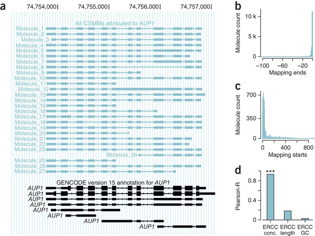
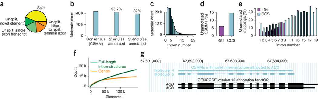
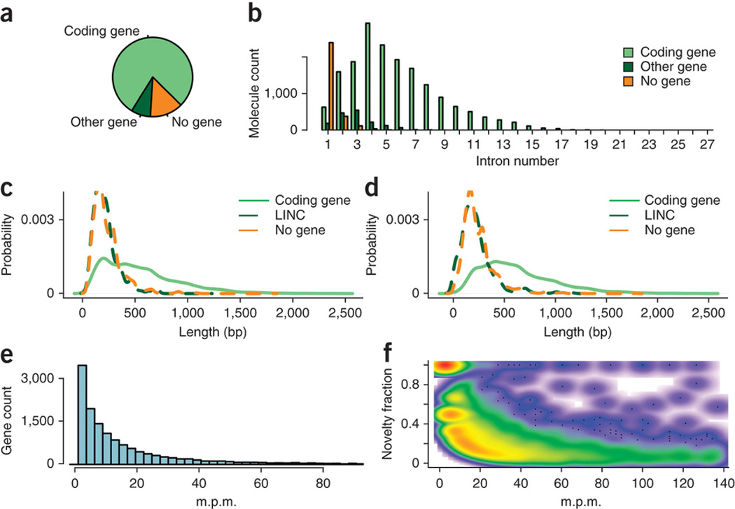
Global RNA studies have become central to understanding biological processes, but methods such as microarrays and short-read sequencing are unable to describe an entire RNA molecule from 5' to 3' end. Here we use single-molecule long-read sequencing technology from Pacific Biosciences to sequence the polyadenylated RNA complement of a pooled set of 20 human organs and tissues without the need for fragmentation or amplification. We show that full-length RNA molecules of up to 1.5 kb can readily be monitored with little sequence loss at the 5' ends. For longer RNA molecules more 5' nucleotides are missing, but complete intron structures are often preserved. In total, we identify ∼14,000 spliced GENCODE genes. High-confidence mappings are consistent with GENCODE annotations, but >10% of the alignments represent intron structures that were not previously annotated. As a group, transcripts mapping to unannotated regions have features of long, noncoding RNAs. Our results show the feasibility of deep sequencing full-length RNA from complex eukaryotic transcriptomes on a single-molecule level.

Figure 1

Completeness of cDNA molecules. (a) Length distribution of GENCODE-annotated transcripts, 454 reads and CCS reads. (b) Distribution of the ratio of the length of each CLR to the length of the CCS read derived from it. (c) Median quality values (QV) for 454 reads and CCS reads as a function of position in the read. (d) HMM polyA calling. Scatterplot of number of nucleotides in polyT state at the beginning of each read (x axis) and number of nucleotides in polyA state at the end of each read (y axis). Color-scale from white (absence of reads) to red (strong enrichment of reads). (e) Pie chart of reads showing four different categories, as defined in the text: g-pA, pT-g, pT-pA and g-g. The first three categories represent polyadenylated molecules, whereas the last category represents molecules lacking a polyA-tail. (f) Length distribution of polyA tails as determined by the HMM, with 19 nt being observed most often. (g) Distribution of distances from the 3′ ends of mappings to annotated transcript end sites (aTES) for polyadenylated molecules, nonpolyadenylated molecules and fragmented RNAs sequenced on a 454 instrument. (h) Distribution of distances from the 5′ ends of mappings to annotated TSS (aTSS) for polyadenylated molecules, nonpolyadenylated molecules and for fragmented RNAs sequenced on a 454 instrument. The black horizontal line represents the median length of 5′ exons of spliced transcripts. (i) Percentage of reads that meet two criteria: (i) the first splice site of the read is the first splice site of an annotated transcript and (ii) the last splice site of the read is the last splice site of an annotated transcript in GENCODE. The observed difference between 454 and CCS reads is statistically significant (two-sided Fisher test, P < 2.2e-16). (j) After calculating the percentage for CCS reads in i for each gene separately, we binned genes by the length of their longest annotated transcript. The plot shows boxplots for ten regularly-spaced bins (from 600–899 bp up to 3,300–3,599 bp) and one bin containing all longer genes. Note that the boundaries of the bins are only shown for every third bin.

Figure 2

Assessment of completeness of CCS reads in controlled environments. (a) All CSMMs (blue) mapping to AUP1 (annotation in black). The only criteria that led to the choice of this example gene were: (i) its most exon–rich transcript had 12 exons and (ii) the genomic distance between gene start and the gene end was ≤4 kb (allowing easy display). (b) Distribution of missing 3′ nucleotides in CCS reads mapped to the original ERCC sequences. (c) Distribution of missing 5′ nucleotides in CCS reads mapped to the original ERCC sequences. (d) Pearson correlation between log-transformed number of CCS reads and log-transformed known ERCC concentration (left), log-transformed ERCC-sequence length (middle) and log transformed GC content of the ERCC sequences. ***P < 0.001 (Pearson correlation t-test – see cor.test in R (ref. 16)).

Figure 3

Exon-intron structure of molecules. (a) Pie-chart indicating the fraction of high confidence mappings that were: split into two or more segments (yellow); unsplit and overlapped no annotated element (darker green); unsplit with strong overlap with an annotated single-exon transcript (lighter green); unsplit with strong overlap of a terminal exon (darker orange); and unsplit overlapping other nonterminal exons (lighter orange). (b) Number of CSMMs having intron-consensus di-nucleotides at the ends of all splits (left), at least one split-end as an annotated splice site for all splits (middle) and only annotated splice sites (right). ss, splice sites. (c) Distribution of number of introns for CSMMs. (d) Percentage of unannotated CSMMs in 454 data and the CCS read data generated in this study. The observed difference is statistically significant (two-sided Fisher test, P < 2.2e-16). (e) Percentage of unannotated mappings for CSMMs with different numbers of introns for 454 and CCS read data. (f) Number of annotated genes (orange) and full-length isoforms (green), based on increasing numbers of CSMMs. (g) Example gene (ACD) with two unannotated isoforms shown by CSMMs. All CSMMs aligned to this gene are shown in Supplementary Figure 4.

Figure 4

Analysis of unannotated transcripts. (a) Pie chart indicating the fraction of molecules corresponding to unannotated isoforms that shared a splice site with a known protein-coding gene (“coding gene”), with another spliced gene class (“other gene”) and those that do not share a splice site with any gene (“no gene”). (b) Same data as in a broken up by intron number in the CSMM mapping. (c) Proteincoding capacity of CSMMs. (d) Same plot as in c but showing the longest uninterrupted coding sequence starting with an ATG for each CSMM. (e) For known genes, we calculated the number of CSMMs that could be attributed to this gene (≥1 splice site in common) per million well-mapped reads (m.p.m.). (f) Scatterplot with m.p.m. on the x axis and the fraction of CSMMs that indicated an unannotated isoform of this gene on the y axis. Color scale from white (absence of molecules) to red (strong enrichment of molecules).

References

1. Nagalakshmi U, et al. The transcriptional landscape of the yeast genome defined by RNA sequencing. Science. 2008;320:1344–1349. - PMC - PubMed
1. Wang ET, et al. Alternative isoform regulation in human tissue transcriptomes. Nature. 2008;456:470–476. - PMC - PubMed
1. Sultan M, et al. A global view of gene activity and alternative splicing by deep sequencing of the human transcriptome. Science. 2008;321:956–960. - PubMed
1. Mortazavi A, Williams BA, McCue K, Schaeffer L, Wold B. Mapping and quantifying mammalian transcriptomes by RNA-Seq. Nat. Methods. 2008;5:621–628. - PubMed
1. Wilhelm BT, et al. Dynamic repertoire of a eukaryotic transcriptome surveyed at single-nucleotide resolution. Nature. 2008;453:1239–1243. - PubMed
Publication types