Binocular stereoscopy in visual areas V-2, V-3, and V-3A of the macaque monkey

Abstract

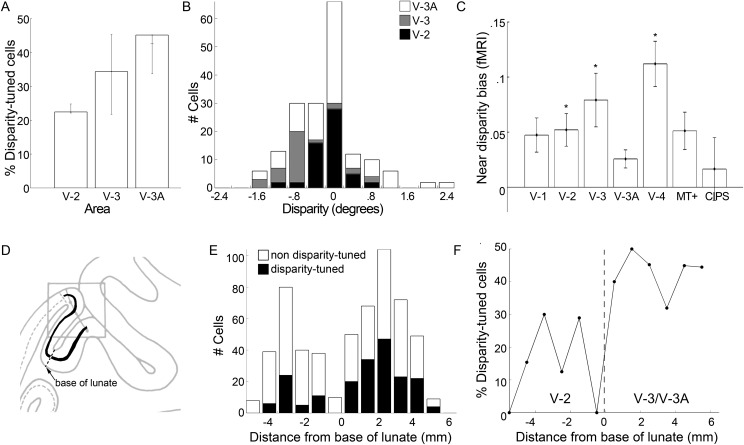
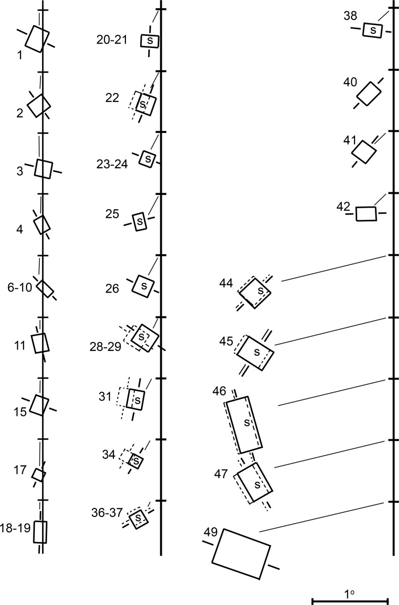
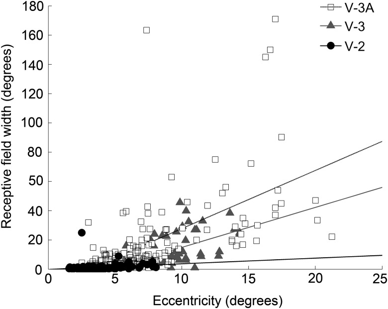
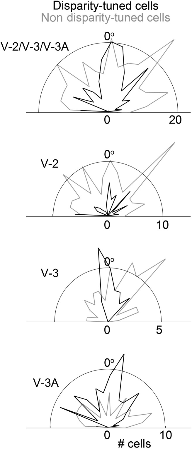
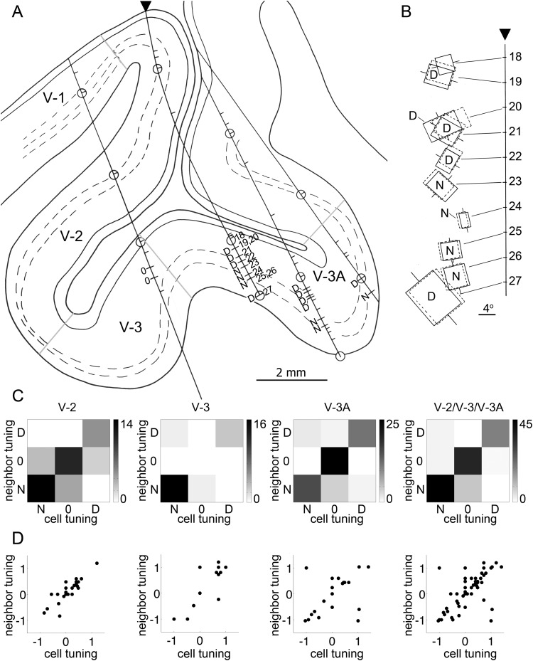
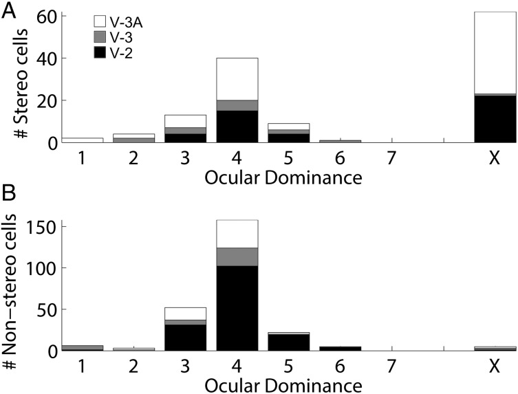
Over 40 years ago, Hubel and Wiesel gave a preliminary report of the first account of cells in monkey cerebral cortex selective for binocular disparity. The cells were located outside of V-1 within a region referred to then as "area 18." A full-length manuscript never followed, because the demarcation of the visual areas within this region had not been fully worked out. Here, we provide a full description of the physiological experiments and identify the locations of the recorded neurons using a contemporary atlas generated by functional magnetic resonance imaging; we also perform an independent analysis of the location of the neurons relative to an anatomical landmark (the base of the lunate sulcus) that is often coincident with the border between V-2 and V-3. Disparity-tuned cells resided not only in V-2, the area now synonymous with area 18, but also in V-3 and probably within V-3A. The recordings showed that the disparity-tuned cells were biased for near disparities, tended to prefer vertical orientations, clustered by disparity preference, and often required stimulation of both eyes to elicit responses, features strongly suggesting a role in stereoscopic depth perception.

Keywords: Hubel and Wiesel, stereopsis; binocular vision; depth; extrastriate cortex; functional organization.

Figure 1.

Bird's eye view of the recording set-up for measuring disparity tuning in macaque extrastriate cortex. See Results and Methods for details.

Figure 2.

Responses of 2 disparity-tuned neurons recorded on 24 June 1969 in what is now known to be V-2 (see Fig. 3). (A) Cell 31, receptive field map. Diagram at the bottom shows the laser beam coordinates of gaze directions indicating aligned eyes, near disparities, and far (distant) disparities. (The dark horizontal band across the page is an acid stain caused by 43-year-old masking tape.) The neuron's peak tuning is indicated in pencil. (B) Cell 31, disparity-tuning curve; squares show responses to single-eye stimulation (solid, right; open, left). (C) Cell 20, responses to horizontal disparities showing maximal activation to aligned LE and RE receptive fields. Dashed lines indicate receptive field for the left eye (LE); solid lines indicate receptive field for the right eye (RE). (D) Cell 20, disparity-tuning curve; single-eye response for each eye shown as a square symbol. Each point in the graph is the average of 10 back-and-forth passes of a computer-generated moving slit. (E) Cell 20, responses to stimulation of either eye alone (top panels), and to both eyes simultaneously (bottom panel). See Supplementary File 1; Supplementary Movies 1–6; Supplementary Figures 1 and 2.

Figure 3.

Reconstruction of electrode penetrations. (A) Low-power, Nissl-stained sagittal section from the experiment run on 24 June 1969. Black arrow shows the area 17/area 18 border. Electrode tract has been drawn on the tracing of the section. The tracing of the cortex within the boxed region of (A) is shown in (B), superimposed on the corresponding MRI macaque atlas section showing area designations. The MRI atlas was generated using different animals from those used in the physiology experiments; the atlas was made by conducting a functional scan of retinotopy to identify area borders (e.g., see Fize et al. 2003). (C) high-resolution Nissl-stained section corresponding to the boxed region in (B), containing the 3 electrolytic lesions made during the recording (arrows). (D) Cell identifications reconstructed on the electrode tract. Red dashes indicate disparity-tuned neurons.

Figure 4.

Reconstruction of the visual areas traversed during 6 experiments (each row from one experiment). Left panels show tracings of the sagittal sections containing the electrode tracts. Regions along the electrode penetration in red are those in which disparity-tuned neurons were identified. Center panels show the matching slice from a monkey atlas of visual areas generated with fMRI. Right panels, overlay.

Figure 5.

Quantification of single-cell results. (A) Proportion of neurons recorded in each visual area selective for binocular disparity. Error bars show upper and lower estimates as predicted from the alignment of the electrode penetrations with the MRI atlas of visual areas. Some electrode penetrations glanced the predicted border between V-3 and V-3A. The upper estimate includes all neurons that could potentially have resided within the visual area; the lower estimate includes only those neurons that were very likely to have resided in the visual area. (B) Population distribution of disparity preferences among extrastriate disparity-tuned neurons. (C) fMRI response to near- versus far-disparity stimuli. Near-disparity bias index was calculated as [(Response to drifting random dot stereograms containing only near disparities − Response to drifting random dot stereograms containing only far disparities)/(Response to drifting random dot stereograms containing only near disparities + Response to drifting random dot stereograms containing only far disparities)]. Asterisk shows a significant bias for near disparities, P < 0.05 (unpaired 2-tailed t-test, N = 4 hemispheres). CIPS: caudal intraparietal sulcus. (D) Tracing of the sagittal section containing the electrode penetration (see Fig. 3B) showing layer 4 (black line) and the base of the lunate sulcus (dashed line), an anatomical landmark that coincides with the border between V-2 and V-3. (E) The total number of disparity-tuned and nondisparity-tuned neurons within 1 mm bins at various distances from the base of the lunate sulcus (negative numbers are within putative V-2; positive numbers are within putative V-3/V-3A). (F) The proportion of neurons that showed disparity tuning recorded at various distances from the base of the lunate sulcus (compare with A).

Figure 6.

Reconstruction of the receptive-field maps for all the neurons encountered on the experiment conducted on 24 June 1969 (see Figs 2 and 3). “S” indicates disparity-tuned (“stereo”) neurons. The horizontal tick marks along the vertical line show the center of gaze. The receptive fields have been splayed out along the vertical axis, so that individual overlapping receptive fields can be easily discriminated. See also Supplementary Figures 3 and 4.

Figure 7.

Receptive field width as a function of the eccentricity of the receptive field within the visual field for neurons recorded in V-2, V-3, and V-3A.

Figure 8.

Orientation preferences for the population of disparity-tuned (black lines) and nondisparity-tuned (gray lines) neurons in V-2, V-3, V-3A, and combined. Neurons selective for vertical bars are plotted at 0°. Supplementary Figure 5 shows results for each cell separately. Supplementary Movie 4 shows tests of the orientation sensitivity of one example neuron.

Figure 9.

Clustering of disparity-tuned neurons by disparity preference (N = near; 0 = zero; D = distant). (A) Tracing of the sagittal slice from an example experiment containing 4 penetrations. Area designations were obtained by aligning the slice with an atlas of visual areas obtained with fMRI. (B) Receptive field reconstructions for neurons 18 through 27 recorded in the second penetration, marked by an arrowhead in (A). The horizontal tick marks along the vertical line show the center of gaze. The receptive fields have been splayed out along the vertical axis, so that individual overlapping receptive fields can be easily discriminated. For cells preferring distant disparity, the cell peaked with the left eye's receptive field (solid line) deviated to the right of the right eye's receptive field (dashed line); for cells preferring near disparity, the optimal stimulus configuration required the left eye's receptive field displaced to the left of the right eye's receptive field. (C) Quantification of spatial clustering by visual area using values binned as either “near,” “distant,” or “zero” disparity preference, as done in the original analysis from around 1970 (see Supplementary Fig. 6). Scale bar shows the number of cells. Spatial clustering is evident in peaks along the y = x axis. (D) Quantification of spatial clustering by visual area. Note that near-disparity preferences are plotted at plus values, following contemporary conventions. Spatial clustering is evident in peaks along the y = x axis. For panels (left to right), the R2 values are 0.77, 0.78, 0.23, and 0.51.

Figure 10.

Responses to monocular versus binocular stimulation. (A) Population distribution of disparity-tuned neurons. Values of “1” correspond to neurons whose responses were entirely driven by the left eye; “7,” correspond to neurons whose responses were entirely driven by the right eye; and “4,” by both eyes equally. Obligate binocular cells, which require simultaneous stimulation of both eyes, are shown in column “X.” (B) Distribution of nondisparity-tuned neurons.

References

1. Adams DL, Zeki S. Functional organization of macaque V3 for stereoscopic depth. J Neurophysiol. 2001;86:2195–2203. - PubMed
1. Anzai A, Chowdhury SA, DeAngelis GC. Coding of stereoscopic depth information in visual areas V3 and V3A. J Neurosci. 2011;31:10270–10282. - PMC - PubMed
1. Backus BT, Fleet DJ, Parker AJ, Heeger DJ. Human cortical activity correlates with stereoscopic depth perception. J Neurophysiol. 2001;86:2054–2068. - PubMed
1. Bakin JS, Nakayama K, Gilbert CD. Visual responses in monkey areas V1 and V2 to three-dimensional surface configurations. J Neurosci. 2000;20:8188–8198. - PMC - PubMed
1. Barlow HB, Blakemore C, Pettigrew JD. The neural mechanism of binocular depth discrimination. J Physiol. 1967;193:327–342. - PMC - PubMed
Publication types