Finite element analysis and CT-based structural rigidity analysis to assess failure load in bones with simulated lytic defects

Abstract

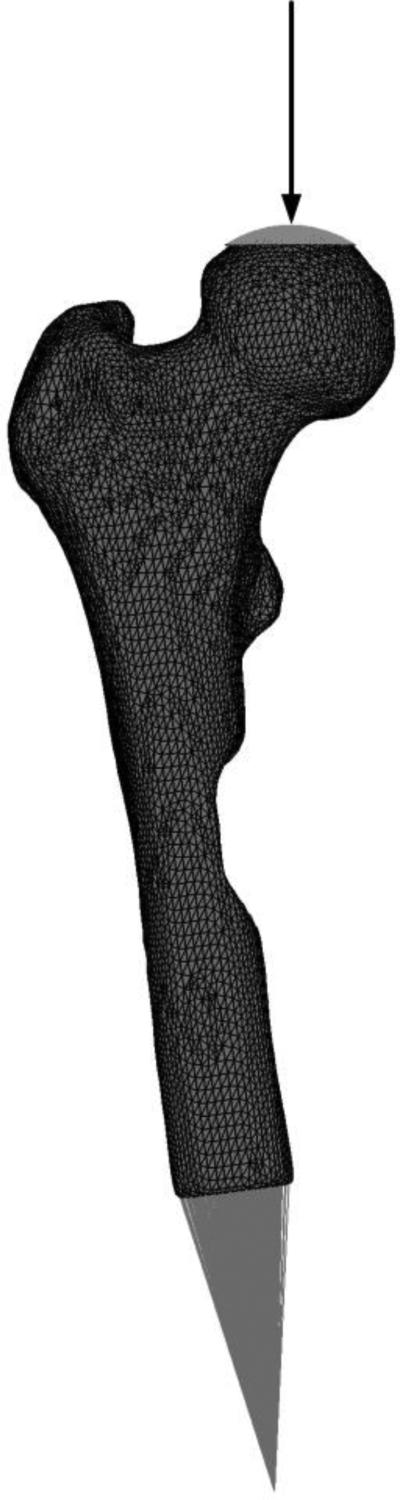
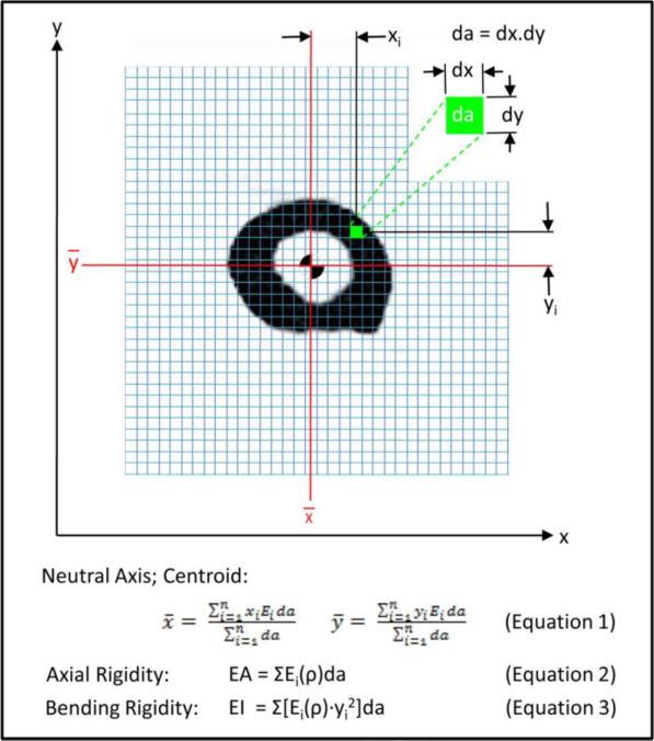
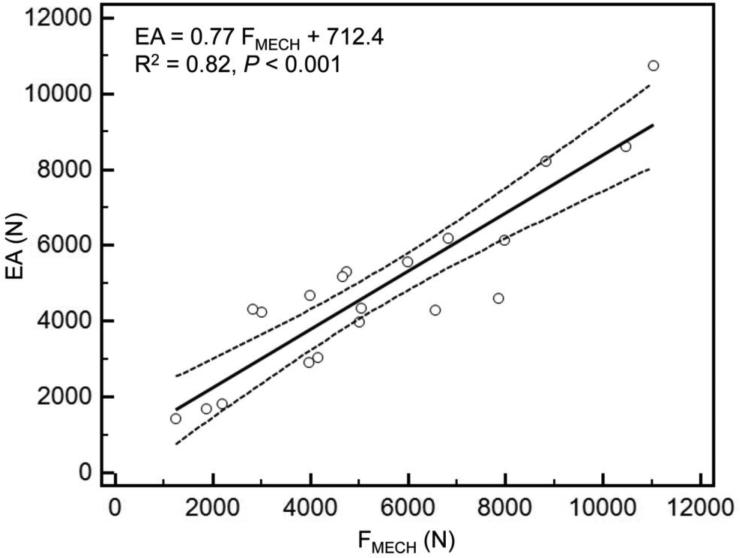
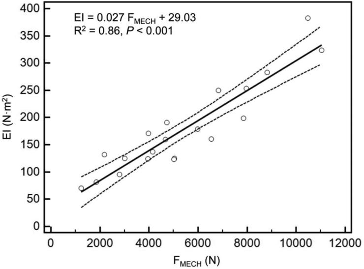
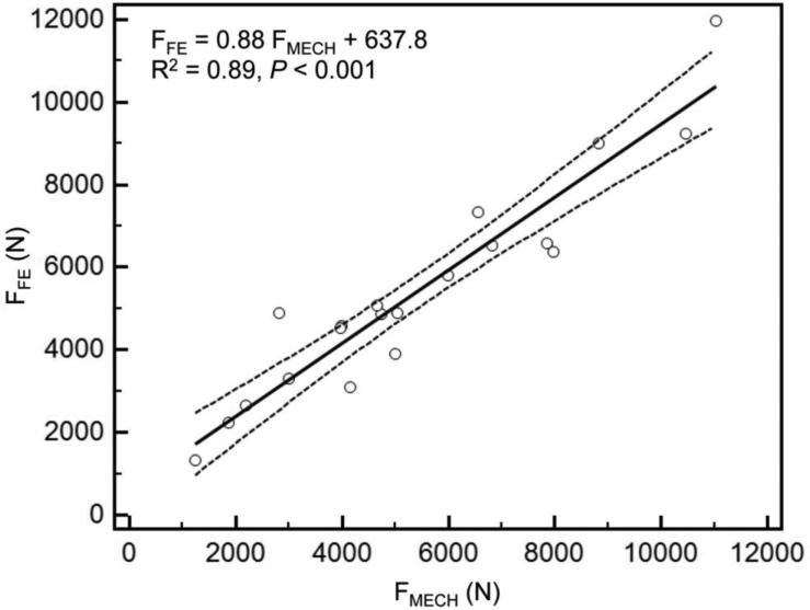
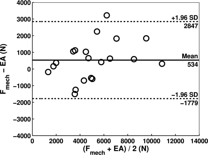
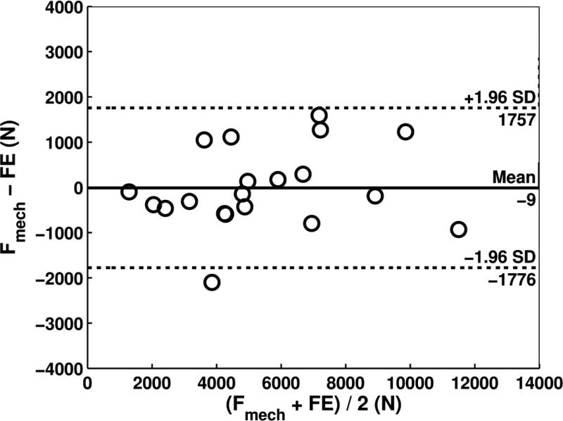
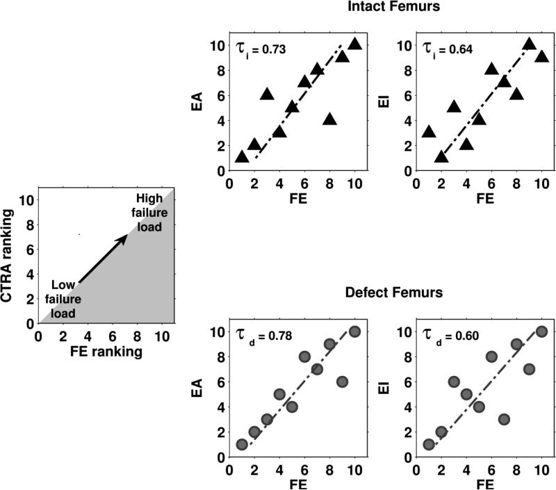
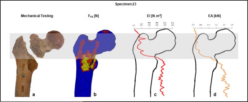
There is an urgent need to improve the prediction of fracture risk for cancer patients with bone metastases. Pathological fractures that result from these tumors frequently occur in the femur. It is extremely difficult to determine the fracture risk even for experienced physicians. Although evolving, fracture risk assessment is still based on inaccurate predictors estimated from previous retrospective studies. As a result, many patients are surgically over-treated, whereas other patients may fracture their bones against expectations. We mechanically tested ten pairs of human cadaveric femurs to failure, where one of each pair had an artificial defect simulating typical metastatic lesions. Prior to testing, finite element (FE) models were generated and computed tomography rigidity analysis (CTRA) was performed to obtain axial and bending rigidity measurements. We compared the two techniques on their capacity to assess femoral failure load by using linear regression techniques, Student's t-tests, the Bland-Altman methodology and Kendall rank correlation coefficients. The simulated FE failure loads and CTRA predictions showed good correlation with values obtained from the experimental mechanical testing. Kendall rank correlation coefficients between the FE rankings and the CTRA rankings showed moderate to good correlations. No significant differences in prediction accuracy were found between the two methods. Non-invasive fracture risk assessment techniques currently developed both correlated well with actual failure loads in mechanical testing suggesting that both methods could be further developed into a tool that can be used in clinical practice. The results in this study showed slight differences between the methods, yet validation in prospective patient studies should confirm these preliminary findings.

Keywords: CT-based structural rigidity analysis; Femur; Finite element analysis; Lytic lesion.

Figure 1

Anterior view of the FE-model, generated from a QCT scan. Displacement was applied to the model via the cup on the head of the femur, while the bottom of the model was fixated by means of high stiffness springs.

Figure 2

Schematic diagram illustrating the pixel-based CTRA analysis algorithm to calculate axial (EA) and bending (EI) rigidities. Each grid element is intended to represent one pixel (the exaggeration of the grid element size is done solely for illustration purposes). The different equations are presented, where ρ represents bone density, x_i and y_i represent the distance of each pixel form the x and y axes respectively, da represents the area of each pixel, E_i represents Young's modulus of elasticity (defined as the ratio of tensile strength to strain in the linear region), and G_i represents the shear modulus (defined as the ratio of shear stress to shear strain in the linear region). The modulus neutral axis and centroid (Equation 1) are determined based on the coordinates of the i^th pixel, its modulus (E_i), area (da), and total number of pixels in the bone cross-section (n). Axial rigidity, which provides a measure of the bone's resistance to deformation when subjected to uniaxial tensile or compressive loads (equation 2), is estimated by summing the products of each pixel's elastic modulus (E_i) and pixel area (da). Bending rigidity provides a measure of the bone's resistance to flexure deformation when subjected to bending moments. Its rigidity about the y-axis (equation 3) is the sum of the products of the elastic modulus (E_i), square of the i^th pixel distance to the neutral axis (ȳ), and the pixel area (da).

Figure 3

A) Linear regression between failure load from mechanical testing versus axial rigidity (a) and bending rigidity (b) and failure load predicted by the FE models (c).

Figure 3

A) Linear regression between failure load from mechanical testing versus axial rigidity (a) and bending rigidity (b) and failure load predicted by the FE models (c).

Figure 3

A) Linear regression between failure load from mechanical testing versus axial rigidity (a) and bending rigidity (b) and failure load predicted by the FE models (c).

Figure 4

Bland-Altman plots for CTRA based axial rigidity (a) and FE based failure load (b). In Figure 4a, the Bland-Altman plot compares the force (N) between mechanical testing and EA for 20 human femurs and shows that the mean difference is 534 N, indicating that on average, force as measured by mechanical testing was 534 N greater than force determined by EA (solid line). The dashed lines represent the 95% limits of agreement and indicate that the difference between the two methods, while averaging 534 N, may range between 1779 N lower to 2847 N higher for mechanical testing compared to EA. There was no significant correlation between the difference on the y-axis and the mean on the x-axis of the two methods, suggesting that the bias is approximately constant throughout the range of values for the 20 human specimens. Regarding Figure 4b, the Bland-Altman plot shows the mean difference in force between mechanical testing and finite element (FE) analysis to be only -9 N, meaning that on average the difference or bias between the two sets of measurements is very close to 0, (ie, about 9 N greater with FE than with mechanical testing). In addition, the limits of agreement as denoted by the dashed lines (+/− 1.96 × SD of the mean difference) reveals that 95% of the time the force using mechanical testing can be somewhere 1776 N lower than FE to 1757 N higher than FE. Again, the bias appears to be constant throughout the range of values, meaning that the variability of the paired measurements between mechanical and FE vary almost equally above and below the mean (solid) line. The Bland-Altman plots in essence provide an excellent graphical representation for assessing agreement between two different methods of measurement and the limits of agreement demarcate the width of the difference that can be expected 95% of the time. The Bland-Altman technique does not require having a “gold standard,” but typically the “new method of interest” (e.g., EA or FE) is subtracted from the conventional method (in this case, mechanical testing) on the y-axis.

Figure 4

Bland-Altman plots for CTRA based axial rigidity (a) and FE based failure load (b). In Figure 4a, the Bland-Altman plot compares the force (N) between mechanical testing and EA for 20 human femurs and shows that the mean difference is 534 N, indicating that on average, force as measured by mechanical testing was 534 N greater than force determined by EA (solid line). The dashed lines represent the 95% limits of agreement and indicate that the difference between the two methods, while averaging 534 N, may range between 1779 N lower to 2847 N higher for mechanical testing compared to EA. There was no significant correlation between the difference on the y-axis and the mean on the x-axis of the two methods, suggesting that the bias is approximately constant throughout the range of values for the 20 human specimens. Regarding Figure 4b, the Bland-Altman plot shows the mean difference in force between mechanical testing and finite element (FE) analysis to be only -9 N, meaning that on average the difference or bias between the two sets of measurements is very close to 0, (ie, about 9 N greater with FE than with mechanical testing). In addition, the limits of agreement as denoted by the dashed lines (+/− 1.96 × SD of the mean difference) reveals that 95% of the time the force using mechanical testing can be somewhere 1776 N lower than FE to 1757 N higher than FE. Again, the bias appears to be constant throughout the range of values, meaning that the variability of the paired measurements between mechanical and FE vary almost equally above and below the mean (solid) line. The Bland-Altman plots in essence provide an excellent graphical representation for assessing agreement between two different methods of measurement and the limits of agreement demarcate the width of the difference that can be expected 95% of the time. The Bland-Altman technique does not require having a “gold standard,” but typically the “new method of interest” (e.g., EA or FE) is subtracted from the conventional method (in this case, mechanical testing) on the y-axis.

Figure 5

The output parameters (failure load for FE and EA and EI for CTRA) were used to rank the femurs from weak to strong. These rankings were subsequently compared by calculating the Kendall rank correlation coefficient (τ). This figure shows Kendall rank correlation coefficients between failure load predicted by the FE models and axial (left panel) and bending (right panel) rigidities calculated by CTRA, both for intact (τ_i , triangles) and metastatic femurs (τ_d , circles).

Figure 6

Fracture location as demonstrated by mechanical testing (a), FE (b) and CTRA analysis (c and d) on a representative specimen. The grey band highlights the failed area as outlined from mechanical testing (panel a). The FE results indicate the elements that underwent plastic deformation in this region (red to yellow sections in panel b), and the bending and axial rigidities (panel c and d) show the lowest EI and EA values for the CT slices residing in the grey fracture zone. The horizontal bar at the top provides the EA and EI axes, and the vertical axis (not shown in axis, which is collinear with the long axis of the bone) is the slice number of the CT data stack.

References

1. Schulman KL, Kohles J. Economic burden of metastatic bone disease in the U.S. Cancer. 2007;109:2334–2342. - PubMed
1. Clezardin P, Teti A. Bone metastasis: pathogenesis and therapeutic implications. Clin Exp Metastasis. 2007;24:599–608. - PubMed
1. Coleman RE. Clinical features of metastatic bone disease and risk of skeletal morbidity. Clin Cancer Res. 2006;12:6243s–6249s. - PubMed
1. Hage WD, Aboulafia AJ, Aboulafia DM. Incidence, location, and diagnostic evaluation of metastatic bone disease. Orthop Clin North Am. 2000;31:515–28, vii. - PubMed
1. Toma CD, Dominkus M, Nedelcu T, Abdolvahab F, Assadian O, Krepler P, Kotz R. Metastatic bone disease: a 36-year single centre trend-analysis of patients admitted to a tertiary orthopaedic surgical department. J Surg Oncol. 2007;96:404–410. - PubMed
Publication types