. 2014 Jun;35(6):2674-97.
doi: 10.1002/hbm.22359. Epub 2013 Oct 23.

Local label learning (LLL) for subcortical structure segmentation: application to hippocampus segmentation

Affiliations

Local label learning (LLL) for subcortical structure segmentation: application to hippocampus segmentation

Yongfu Hao et al. Hum Brain Mapp. 2014 Jun.

Abstract

Automatic and reliable segmentation of subcortical structures is an important but difficult task in quantitative brain image analysis. Multi-atlas based segmentation methods have attracted great interest due to their promising performance. Under the multi-atlas based segmentation framework, using deformation fields generated for registering atlas images onto a target image to be segmented, labels of the atlases are first propagated to the target image space and then fused to get the target image segmentation based on a label fusion strategy. While many label fusion strategies have been developed, most of these methods adopt predefined weighting models that are not necessarily optimal. In this study, we propose a novel local label learning strategy to estimate the target image's segmentation label using statistical machine learning techniques. In particular, we use a L1-regularized support vector machine (SVM) with a k nearest neighbor (kNN) based training sample selection strategy to learn a classifier for each of the target image voxel from its neighboring voxels in the atlases based on both image intensity and texture features. Our method has produced segmentation results consistently better than state-of-the-art label fusion methods in validation experiments on hippocampal segmentation of over 100 MR images obtained from publicly available and in-house datasets. Volumetric analysis has also demonstrated the capability of our method in detecting hippocampal volume changes due to Alzheimer's disease.

Keywords: SVM; hippocampal segmentation; local label learning; multi-atlas based segmentation.


Figures

Figure 1
Figure 1
The framework of local label learning (LLL) method, consisting of steps: (1) candidate training set construction, (2) feature extraction, and (3) local SVM classification. [Color figure can be viewed in the online issue, which is available at http://wileyonlinelibrary.com.]
Figure 2
Figure 2
Feature extraction for a randomly selected image by applying filters with different parameters. The displayed filtering outputs are scaled to have the same intensity range as the intensity indicator.
Figure 3
Figure 3
The initial segmentation result of a randomly selected test image based on the probabilistic voting. The first row shows three slices of the test image with manual segmentation label. The probabilistic voting results are shown in the second row and the color bar indicates the probability of a voxel belonging to the hippocampus. The voxels belonging to the hippocampus or not with 100% certainty (probability value is 1: red or 0: blue) are overlaid on the test image in the third row. First column: horizontal; second column: sagittal; third column: coronal. [Color figure can be viewed in the online issue, which is available at http://wileyonlinelibrary.com.]
Figure 4
Figure 4
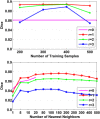
The average Dice index values of segmentation results of the right hippocampus for dataset A with different numbers of training samples and r varying from 0 to 3. Top: SVM classifier based segmentation results. Bottom: kNN classifier based segmentation results. For the SVM classifier based segmentation, all available training samples (20 in total) were used without selection when r = 0. For the kNN classifier based segmentation, all available training samples were used. [Color figure can be viewed in the online issue, which is available at http://wileyonlinelibrary.com.]
Figure 5
Figure 5
Frequency of features used in the segmentation. (1) One randomly selected image with the hippocampus boundary voxels shown in different colors. (2) Features selected in the segmentation. Each row indexed by the color bar shown at the left corresponds to the boundary voxel in the same color shown in (1). The x‐axis is the feature index (1–27: intensity features in the neighborhood of 3×3×3, 1–125: intensity features in the neighborhood of 5×5×5, 1:343: intensity features in the neighborhood of 7×7×7, 344–367: filtering outputs). (3) Frequency of features selected for the segmentation of the image shown in (1). (4) Mean of frequencies of features selected for the segmentation of images of dataset A. [Color figure can be viewed in the online issue, which is available at http://wileyonlinelibrary.com.]
Figure 6
Figure 6
Box plots of the results for the dataset A. On each box, the central mark is the median, and edges of the box are the 25th and 75th percentiles. Whiskers extend from each end of the box to the adjacent values in the dataset and the extreme values within 1 interquartile range from the ends of the box. Outliers are data with values beyond the ends of the whiskers. [Color figure can be viewed in the online issue, which is available at http://wileyonlinelibrary.com.]
Figure 7
Figure 7
Box plots of the results for the dataset B. On each box, the central mark is the median, and edges of the box are the 25th and 75th percentiles. Whiskers extend from each end of the box to the adjacent values in the dataset and the extreme values within 1 interquartile range from the ends of the box. Outliers are data with values beyond the ends of the whiskers. [Color figure can be viewed in the online issue, which is available at http://wileyonlinelibrary.com.]
Figure 8
Figure 8
Box plots of the results for the dataset C. On each box, the central mark is the median, and edges of the box are the 25th and 75th percentiles. Whiskers extend from each end of the box to the adjacent values in the dataset and the extreme values within 1 interquartile range from the ends of the box. Outliers are data with values beyond the ends of the whiskers. [Color figure can be viewed in the online issue, which is available at http://wileyonlinelibrary.com.]
Figure 9
Figure 9
Relative volume differences (RVD) (first row) and absolute value of RVD (ARVD) (second row) between the segmentation results of automatic methods and the manual label on the three datasets. Figures at the right side are the zoomed in version of figures at the left side. On each box, the central mark is the median, and edges of the box are the 25th and 75th percentiles. Whiskers extend from each end of the box to the adjacent values in the dataset and the extreme values within 1 times the interquartile range from the ends of the box. Outliers are data with values beyond the ends of the whiskers. [Color figure can be viewed in the online issue, which is available at http://wileyonlinelibrary.com.]
Figure 10
Figure 10
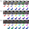
Hippocampal segmentation results obtained by different methods. One subject was randomly chosen from each dataset. For each subject, the first row shows the segmentation results produced by different methods, the second row demonstrates their corresponding surface rendering results, and the difference between results of manual and automatic segmentation methods was showed in the third row (red: manual segmentation results, green: automated segmentation results, blue: overlap between manual and automated segmentation results). [Color figure can be viewed in the online issue, which is available at http://wileyonlinelibrary.com.]
Figure 11
Figure 11
Hippocampal volumes of subjects from three diagnostic groups. On each box, the central mark is the median, and edges of the box are the 25th and 75th percentiles. Whiskers extend from each end of the box to the adjacent values in the dataset and the extreme values within 1 interquartile range from the ends of the box. Outliers are data with values beyond the ends of the whiskers. [Color figure can be viewed in the online issue, which is available at http://wileyonlinelibrary.com.]
Figure 12
Figure 12
Segmentation performance as a function of the number of atlases used. [Color figure can be viewed in the online issue, which is available at http://wileyonlinelibrary.com.]
Figure 13
Figure 13
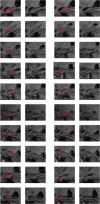
Ten randomly selected images and their segmentation labels of hippocampus obtained from the results provided by the study [Heckemann et al., 2011]. Each row shows one image's two slices and their corresponding segmentation labels. [Color figure can be viewed in the online issue, which is available at http://wileyonlinelibrary.com.]

Similar articles

Cited by

References

    1. Aljabar P, Heckeman R, Hammers A, Hajnal JV, Rueckert D (2007): Classifier selection strategies for label fusion using large atlas databases. Med Image Comput Comput Assist Interv 4791:523–531. - PubMed
    1. Aljabar P, Heckemann RA, Hammers A, Hajnal JV, Rueckert D (2009): Multi‐atlas based segmentation of brain images: Atlas selection and its effect on accuracy. Neuroimage 46:726–738. - PubMed
    1. Artaechevarria X, Munoz‐Barrutia A, Ortiz‐de‐Solorzano C (2008): Effleient classifier generation and weighted voting for aflas‐based segmentation: Two small steps faster and closer to the combination oracle. SPIE Med Imag 2008:6914.
    1. Artaechevarria X, Munoz‐Barrutia A, Ortiz‐de‐Solorzano C (2009): Combination strategies in multi‐atlas image segmentation: Application to brain MR data. IEEE Trans Image Process 28:1266–1277. - PubMed
    1. Ashburner J, Friston KJ (2005): Unified segmentation. Neuroimage 26:839–851. - PubMed

Publication types