Detecting range expansions from genetic data

Abstract

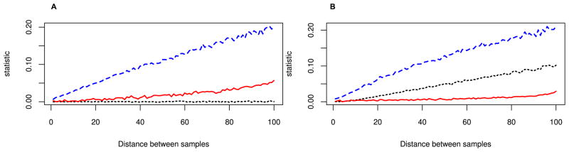
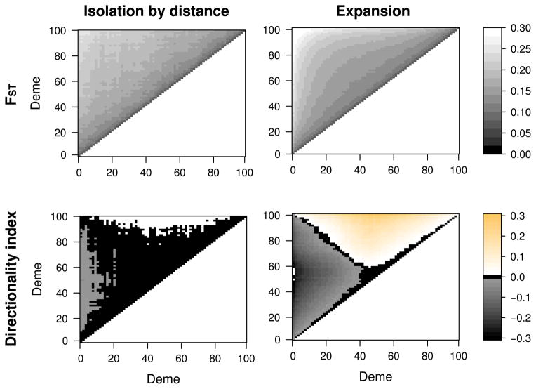
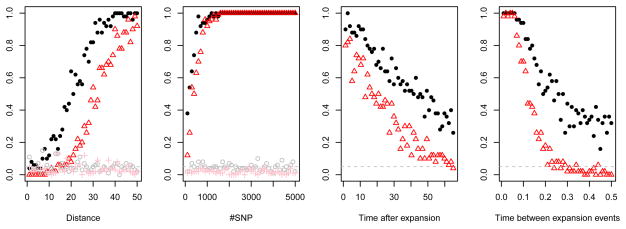
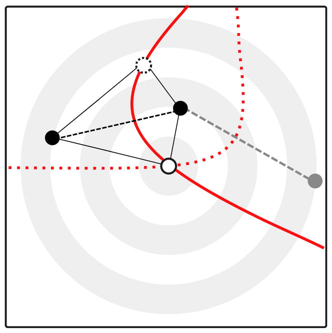
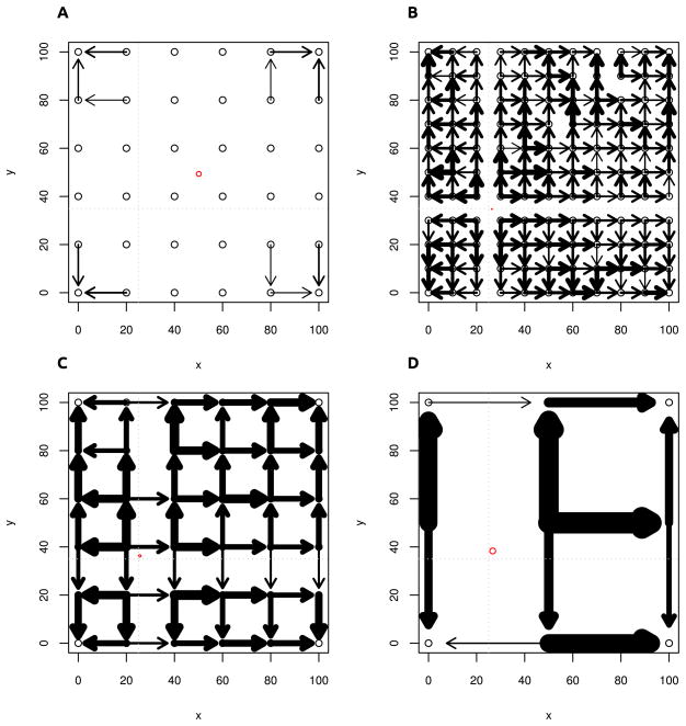
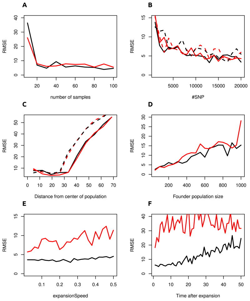
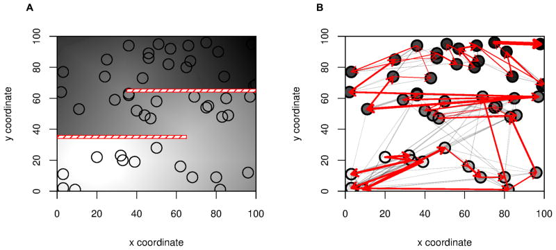
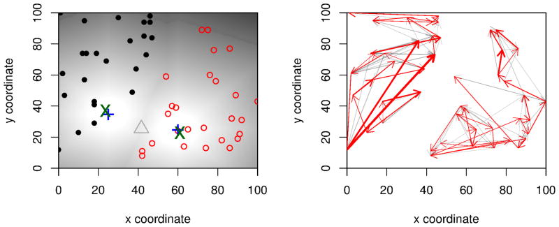
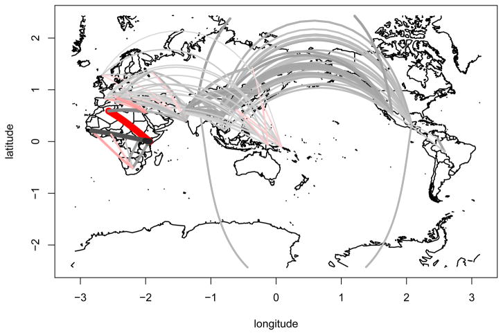
We propose a method that uses genetic data to test for the occurrence of a recent range expansion and to infer the location of the origin of the expansion. We introduce a statistic ψ (the directionality index) that detects asymmetries in the 2D allele frequency spectrum of pairs of population. These asymmetries are caused by the series of founder events that happen during an expansion and they arise because low frequency alleles tend to be lost during founder events, thus creating clines in the frequencies of surviving low-frequency alleles. Using simulations, we show that ψ is more powerful for detecting range expansions than both FST and clines in heterozygosity. We also show how we can adapt our approach to more complicated scenarios such as expansions with multiple origins or barriers to migration and we illustrate the utility of ψ by applying it to a data set from modern humans.

Keywords: Biogeography; evolutionary genomics; gene flow; genetic variation; population structure.

Figure 1. Behavior of H (red, full line), ψ (black, dotted) and F_ST (blue, dashed) in one-dimensional (A) isolation-by-distance and (B) population-expansion models

Simulations were performed on a 200 demestepping-stone model with scaled migration rate M=100 between adjacent demes, and expansion events every 0.001 coalescence units. F_ST increases linearly with distance in both models and ψ is zero in the isolation-by-distance model, but increases approximately linearly in the expansion model. Heterozygosity is plotted for demes from the center of the population (left) to the border of the habitat (right), and given as the difference to the central deme.

Figure 2. Behavior of F_ST and ψ in isolation-by-distance and population expansion model

Each panel gives the value of the pairwise statistics F_ST and ψ under an isolation-by-distance model and an expansion model with the expansion starting in the central deme (50,50). Simulations were performed on a 101 × 101 deme stepping stone model, and a diagonal transect from demes at coordinates (0,0) to (100,100) was sampled, and all pairwise statistics were calculated. Black regions correspond to regions where F_ST and ψ are very low (below 1%). The orange and grey regions denote areas with positive and negative ψ, respectively. Whereas F_ST behaves qualitatively similar under both models, the behavior of ψ is very different. Under isolation-by-distance, ψ is very close to zero, with some deviations due to boundary effects. Under an expansion, however, we see a clear signal for all demes, except demes that are very close to each other, or demes that have the same distance to the origin, but in different directions.

Figure 3. True/false positive rates of detecting range expansion

Each panel give the proportion of replicates in which the null model was rejected at the 5% significance level. Black circles correspond to ψ under an expansion model and an isolation-by-distance model, red triangles and plus signs denote simulations correspond to using H to distinguish an expansion model and isolation by distance model, respectively. The grey dashed line at 0.05 gives the expected proportion of false positives under the null hypothesis. Baseline parameters for the simulations were of 2 chromosomes (one diploid individual) at each location sampled, with locations a distance of 50 each other. Fixed parameters used for generating the data sets are 1,000 independent SNP from one diploid individual per sampled deme. Time between expansion events was set to 0.1 (coalescence units) and the data was observed immediately after the expansion ended.

Figure 4. Illustration of the method used to infer the origin of a range expansion

The black and grey points correspond to genetic samples taken, the white point corresponds to the (unknown) origin of the expansion. Using the directionality index ψ, we can infer the difference in distance from the samples to the origin (dashed lines). The set of all points that has the same difference in distance to the origin corresponds to the arm of a hyperbola (red), which comprises all candidate points according to ψ and the location of two points. Using a second pair of points (the grey and top black point), we can identify a second hyperbola (dotted), and find an unique location of the origin. In practice, we use more than three sampling locations. Sampling noise will cause the hyperbolas to not intersect in a single point and we use a least-squares criterion to estimate the location of the origin.

Figure 5. Detecting the origin of a range expansion

Each panel corresponds to a 101 × 101 grid of populations that were simulated. The expansion began at point (25,35) (indicated by gray dotted lines). Black bordered circles indicate sampling locations, black arrows correspond to ψ > 1% between adjacent samples, with the direction of the arrow indicating the sign of ψ. Thicker arrows correspond to larger ψ. The red ellipse corresponds to the 95% confidence interval of the estimated location of the origin. Panel a: no expansion (isolation-by-distance model). Edge effects cause the estimated origin to be close to the center of the grid of populations. Panels b–d: Expansion with parameters M = 1, t = 0.1 and samples taken every 10th, 20th and 50th deme. While the confidence region is larger for smaller numbers of samples, we get a very accurate result even when we have only 9 samples.

Figure 6. Performance of TDOA method

We present the root mean squared errors (RSME) of our TDOA method (black) compare it with the method of Ramachandran et al. 2005 (red). Samples taken on a grid ware represented by full lines, whereas dashed lines denote samples that were taken from random coordinates in the simulated region. Our method is superior when the expansion occurred slowly or when it finished some time in the past; but the method perform very similar for recent, fast expansions.

Figure 7. Identifying complex patterns of migration

We simulated data on a S-shaped habitat with two impermeable barriers (Panel A) The darkness of the shading is proportional to the arrival time of the expansion, which began in deme (20,20). Black circles correspond to locations sampled. In Panel B we show the inferred pairwise directionality, with all edges remaining after thinning the graph shown in grey, and a maximum spanning tree in red. We also show the inferred ordering of the samples as a color gradient of the samples from light (closest to origin) to dark. The barriers can be identified from panel B by the absence of any indication of gene flow across the barriers and by examining the ordering of the samples.

Figure 8. Detecting multiple origins

Panel a: We simulated two expansions that originated at the same time from origins indicated by the blue crosses. The color gradient in the background corresponds to the time of colonization time of each deme. We address the problem of inferring the origin of multiple expansions using a two-step procedure. First, we cluster the samples into discrete clusters (red and black circles, respectively) and then estimate the expansion signal and origins independently for the clusters, resulting in high accuracy for both estimated origins (green X) when compared to the actual origins (blue +). The grey triangle denotes the estimated single origin if we did not do the two step procedure; it lies approximately half way between the two actual origins. The right panel shows the inferred migration patterns after a transitive reduction (grey/red arrows) and a maximum spanning tree (red arrows).

Figure 9. Inference of human migration routes

The figure shows a visual representation of the pairwise directionality indices between human populations in HGDP and HapMap. Each line corresponds to the pairwise ψ statistic, with thicker and brighter lines corresponding to higher values. Grey and red lines denote eastward and westward migration, respectively. Lines with an absolute Z-score below 5 were omitted.

References

-
- Aho AV, Garey MR, Ullman JD. The Transitive Reduction of a Directed Graph. SIAM Journal on Computing. 1972;1:131–137. URL http://epubs.siam.org/doi/abs/10.1137/0201008. - DOI
- Altshuler DM, Gibbs RA, Peltonen L, Dermitzakis E, Schaffner SF, Yu F, Bonnen PE, De Bakker PI, Deloukas P, Gabriel SB. Integrating common and rare genetic variation in diverse human populations. Nature. 2010;467:52. URL http://europepmc.org/articles/PMC3173859. - PMC - PubMed
- Austerlitz F, Jung-Muller B, Godelle B, Gouyon PH. Evolution of coalescence times, genetic diversity and structure during colonization. Theoretical Population Biology. 1997;51:148–164.
- Balakrishnan V, Sanghvi LD. Distance between Populations on the Basis of Attribute Data. Biometrics. 1968;24:859–865. URL http://www.jstor.org/stable/2528876. ArticleType: research-article/Full publication date: Dec., 1968/Copyright © 1968 International Biometric Society.
- Beaumont MA, Zhang W, Balding DJ. Approximate Bayesian computation in population genetics. Genetics. 2002;162:2025–2035. URL http://www.ncbi.nlm.nih.gov/pubmed/12524368. - PMC - PubMed
Publication types
MeSH terms
Grants and funding
LinkOut - more resources
Full Text Sources
Other Literature Sources
Miscellaneous