System identification of the nonlinear dynamics in the thalamocortical circuit in response to patterned thalamic microstimulation in vivo

Abstract

Objective: Nonlinear system identification approaches were used to develop a dynamical model of the network level response to patterns of microstimulation in vivo.

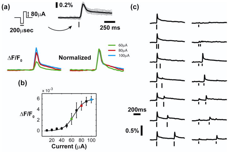
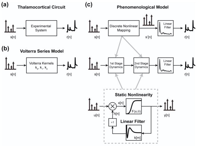
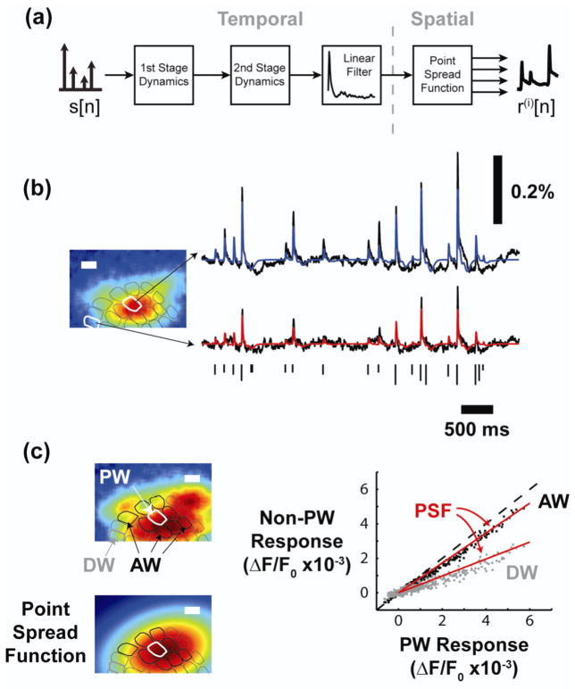
Approach: The thalamocortical circuit of the rodent vibrissa pathway was the model system, with voltage sensitive dye imaging capturing the cortical response to patterns of stimulation delivered from a single electrode in the ventral posteromedial thalamus. The results of simple paired stimulus experiments formed the basis for the development of a phenomenological model explicitly containing nonlinear elements observed experimentally. The phenomenological model was fit using datasets obtained with impulse train inputs, Poisson-distributed in time and uniformly varying in amplitude.

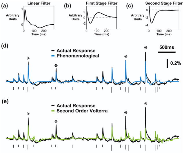
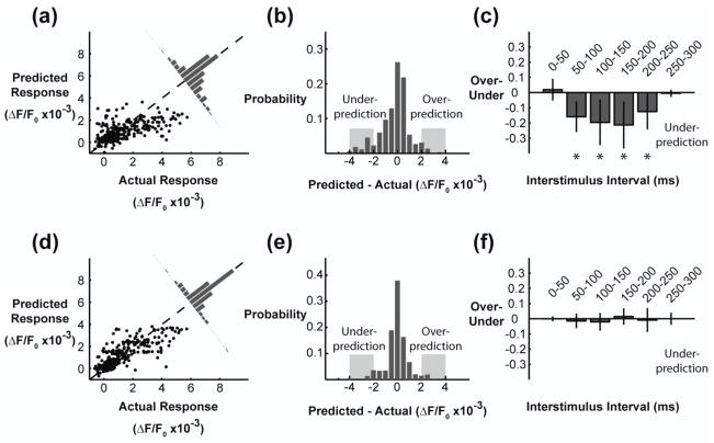
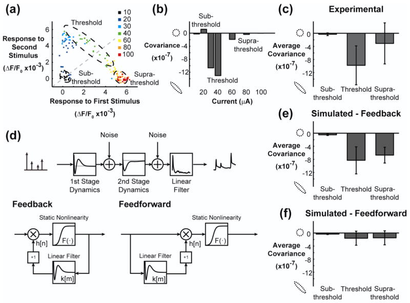
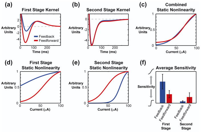
Main results: The phenomenological model explained 58% of the variance in the cortical response to out of sample patterns of thalamic microstimulation. Furthermore, while fit on trial-averaged data, the phenomenological model reproduced single trial response properties when simulated with noise added into the system during stimulus presentation. The simulations indicate that the single trial response properties were dependent on the relative sensitivity of the static nonlinearities in the two stages of the model, and ultimately suggest that electrical stimulation activates local circuitry through linear recruitment, but that this activity propagates in a highly nonlinear fashion to downstream targets.

Significance: The development of nonlinear dynamical models of neural circuitry will guide information delivery for sensory prosthesis applications, and more generally reveal properties of population coding within neural circuits.

Figure 1. Voltage sensitive dye imaging captures the cortical response with high spatial and temporal resolution

(a) Diagram of the imaging system. The electrode is positioned in a “barreloid” in the thalamus, a collection of cells that respond most vigorously to a common whisker. Imaging in cortex captures the response of each cortical column. (b) Histological analysis provides an anatomical map of the cortical column structure (see methods). (c) The anatomical map is aligned to the VSDI image through a least squares mapping to functional data. (d) The cortical response to electrical microstimulation of the thalamus begins ~5–10 milliseconds after stimulation, but quickly grows in amplitude and spreads spatially. Scale bars in (b), (c), and (d) are 500 micrometers.

Figure 2. Microstimulation of the thalamus produces a nonlinear cortical response

(a) Top: By averaging within a single cortical column, we obtain a timecourse of cortical activation with high signal to noise ratio. The “tick” represents the presentation time of the stimulus, which is a symmetric biphasic current waveform. The height of the “ticks” throughout the paper indicates the current amplitude of the stimulus. Microstimulation elicited a characteristic timecourse in the cortical response (single trials in gray, trial-averaged response in black). Bottom: When normalized by the amplitude of the response, the timecourse was consistent across a wide range of stimulus intensities and response amplitudes. (b) The amplitude of the cortical response displayed a nonlinear relationship with the current intensity of the single electrical stimulus. The currents used in (a) are color-coded in (b) for reference. (c) Microstimulation of the thalamus engaged two sets of nonlinear dynamics. A strong electrical stimulus suppressed the response to a second electrical stimulus, with the suppression decreasing for long inter-stimulus intervals. A weak electrical stimulus, however, caused profound facilitation of the response to the second stimulus. This facilitation principally occurs for inter-stimulus intervals of 100–200 milliseconds.

Figure 3. Nonlinear modeling architecture

(a) The goal of the study was to create a nonlinear dynamical model of the response of the thalamocortical circuit to patterns of thalamic microstimulation. A train of microstimulation pulses was delivered as the input, while a continuously varying signal, generated by averaging within a single cortical column, was used as the output. (b) A second order Volterra series model was developed in an attempt to capture the dynamics of the system. The kernels of the model mapped trains of discrete inputs to continuously varying signals. (c) Top: The phenomenological model was developed according to experimental observations described in Figure 2. The response of the system was similar in shape, regardless of stimulus or response amplitude, allowing separation of the model into a nonlinear mapping of discrete impulses followed by a linear filter. Middle: Further, two distinct sets of dynamics were observed and directly incorporated into the model architecture. Bottom: Each of the two stages within the model was comprised of a canonical unit, in which the static and dynamic nonlinearity were independently modeled and parameterized.

Figure 4. Phenomenological model based on experimental observations accurately predicted the cortical response to patterned microstimulation

The average (a) linear kernel, (b) first stage feedback kernel, and (c) second stage feedback kernel of the phenomenological model fit on Poisson train stimuli and VSDI response data (N=7). In each case, the first stage kernel implemented the facilitation dynamics and the second stage implemented the suppression dynamics. (d) An example of the performance of the phenomenological model (blue), with the actual response shown in black. (e) An example of the second order Volterra model performance (green), with the actual response shown in black. In (d) and (e), the height of the ticks indicates the current intensity and the asterisks mark stimuli for which the Volterra model severely under-predicted the response. The phenomenological model performed better for these responses.

Figure 5. Phenomenological model improved error residuals compared to the Volterra model

(a) Error residuals for the second order Volterra model fit via cross-correlation. Each data point is the response to a single stimulus in the RAP stimulus train. (b) The residual distribution had a heavy tail towards under-prediction. (c) The responses were systematically under-predicted for stimuli separated in time by 50–250 milliseconds. (d) Error residuals for the phenomenological model. (e) The residual distribution shows few large errors (indicated by the gray regions) and no bias towards under-prediction or over-prediction. (f) The responses were not systematically under-predicted or over-predicted for any interstimulus intervals.

Figure 6. Extension of phenomenological model captures spatial spread

(a) A linear point spread function, modeled as a two dimensional Gaussian, was used to extend the model spatially across all cortical columns. (b) The spatial extension to the model captured the dynamics for the principal cortical column as well as distant cortical columns. (c) A representative cortical response (top left) and the point spread function (bottom left) were similar. In the scatter plot, the point spread function (red) captures the relative response properties of the principal cortical column and adjacent cortical column for neighboring (black) and distant (gray) cortical columns. Each data point indicates the response to a single impulse within the RAP impulse train. Scale bars in (b) and (c) are 500 micrometers.

Figure 7. Phenomenological model with feedback reproduced single trial variability in facilitation and suppression

(a) The response to the second stimulus (ISI = 150ms) is plotted against the response to the first stimulus for experimental data. The color of each point indicates the current intensity in units of microamperes. The unity line is shown in gray. (b) The trial by trial covariance in the response to the two stimuli was calculated for each stimulus intensity. At sub-threshold and supra-threshold currents, the covariance between the first and second response was low. At a threshold current, there was a strong negative covariance between the first and second response. (c) The negative covariance at the threshold current was consistent across animals. (d) The phenomenological model was used to simulate an identical experiment. The simulated data was created by injecting noise into the model at the output of the first and second stages during presentation of stimuli. A feedback model (same as in Figure 5, displayed in bottom-left of the panel) and a feedforward model (fit specifically for this analysis, displayed in the bottom-right of the panel) were used. Both models utilized a two-stage model architecture, where each stage consisted of a canonical unit. The canonical unit for the feedback (left) and feedforward (right) model are shown in this panel. (e) The feedback model reproduced the strong negative covariance at the threshold current and recovers for supra-threshold currents, and was not significantly different from the experimental data in (c) (p = 0.89, N=7, two-sided paired Student’s t-test). (f) The feedforward model did not reproduce the negative covariance for threshold currents, and the difference from the experimental data was statistically significant (p = 0.003, N=7, two-sided paired Student’s t-test).

Figure 8. Model parameters predict linear local response properties, but nonlinear propagation of activity

(a) The average first stage kernel from the phenomenological model fit with feedback (red) and feedforward (blue) dynamics. (b) The average second stage kernel. (c) An example of the full static nonlinearity created by combining both stages. (d) and (e) The static nonlinearity at the first and second stages, respectively, for the feedback and feedforward models. (f) The average sensitivity across animals (N=7) is distinctly different for the feedback and feedforward models. The feedback model was weakly sensitive in the first stage and highly sensitive in the second stage. The feedforward model was moderately sensitive in both stages.

References

1. Alonso JM, Usrey WM, Reid RC. Precisely correlated firing in cells of the lateral geniculate nucleus. Nature. 1996;383(6603):815–819. - PubMed
1. Bach-y-Rita P, Collins CC, Saunders FA, White B, Scadden L. Vision substitution by tactile image projection. Nature. 1969;221(5184):963–964. - PubMed
1. Barros CG, Bittar RS, Danilov Y. Effects of electrotactile vestibular substitution on rehabilitation of patients with bilateral vestibular loss. Neurosci Lett. 2010;476(3):123–126. - PubMed
1. Bazhenov M, Timofeev I, Steriade M, Sejnowski TJ. Computational Models of Thalamocortical Augmenting Responses. The Journal of Neuroscience. 1998;18(16):6444–6465. - PMC - PubMed
1. Brugger D, Butovas S, Bogdan M, Schwarz C. Real-Time Adaptive Microstimulation Increases Reliability of Electrically Evoked Cortical Potentials. Biomedical Engineering, IEEE Transactions on. 2011;58(5):1483–1491. - PubMed
Publication types
LinkOut - more resources