Cortical high-density counterstream architectures

Abstract

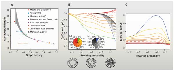
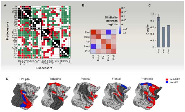
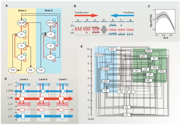
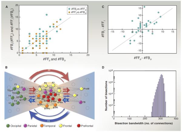
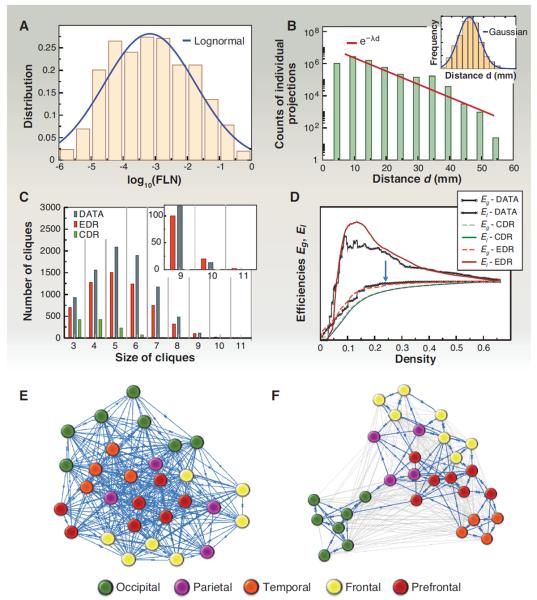
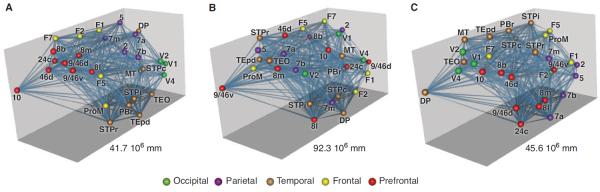
Small-world networks provide an appealing description of cortical architecture owing to their capacity for integration and segregation combined with an economy of connectivity. Previous reports of low-density interareal graphs and apparent small-world properties are challenged by data that reveal high-density cortical graphs in which economy of connections is achieved by weight heterogeneity and distance-weight correlations. These properties define a model that predicts many binary and weighted features of the cortical network including a core-periphery, a typical feature of self-organizing information processing systems. Feedback and feedforward pathways between areas exhibit a dual counterstream organization, and their integration into local circuits constrains cortical computation. Here, we propose a bow-tie representation of interareal architecture derived from the hierarchical laminar weights of pathways between the high-efficiency dense core and periphery.

Fig. 1. High density of the cortical graph excludes sparse small-world architecture

(A) Comparison of the average shortest path length and density of the G_29x29 subgraph with the graphs of previous studies. Sequential removal of weak connections causes an increase in the characteristic path-length. Black triangle: G_29x29; gray area: 95% confidence interval following random removal of connections from G_29x29. Dotted horizontal lines indicate the 5 to 95% interval with at least one unreachable node (after repeated and graded, random edge removal). The three least dense graphs are near their 5% unreachability levels. Data incompleteness meant that some of the initial networks have unreachable nodes (the latter are removed and not considered here); 14 unreachable nodes are from Modha and Singh (44); 1 unreachable node is from Young (43); and 2 unreachable nodes are from Felleman and Van Essen (17). Modha and Singh 2010: (44); Young 1993: (43); Honey et al., 2007: (34); Felleman and Van Essen 1991: (17); Jouve et al., 1998: (45); Markov et al., 2012: (8). “Jouve et al., 1998 predicted” indicates values of the graph inferred using the published algorithm (45). (B) Effect of density on Watts and Strogatz's formalization of the small world. Clustering and average path-length variations generated by edge rewiring with probability range indicated on the x axis applied to regular lattices [of 1000 nodes in a 1D ring as in (31)] of increasingly higher densities. The pie charts show graph density encoded via colors for path length (L) and clustering (C). On the y axis, we indicate the average path length ratio (Lp/Lo) and clustering ratio (Cp/Co) of the randomly rewired network, where Lo and Co are the path length (Lo) and clustering (Co) of the regular lattice, respectively. Lp and Cp are the same quantities measured for the network rewired with probability (p). Hence, for each density value indicated in the L and C pie charts, the corresponding Lp/Lo and Cp/Co curves can be identified. Three diagrams below the x axis indicate the lattice (left), sparsely rewired (middle), and the randomized (right) networks. (C) The small-world coefficient $\frac{Cp∕Co}{Lp∕Lo}$ (33, 136) corresponding to each lattice rewiring. Color code is the same as in (B). Dashed lines in (B) and (C) indicate 42% and 48% density levels. For electronic data files, see www.core-nets.org.

Fig. 2. Binary specificity in the dense network

(A) The G29×29 subgraph adjacency matrix organized so as to illustrate the connectivity within (black squares) and between regions (in green). In red, new-found projections (NFPs). (B) Regional in-link similarity of binary connections; positive values indicate positive correlation and negative values indicate anticorrelation between area pairs, within and between regions. The diagonal corresponds to average intraregion similarity; everywhere else is interregion similarity. Occ, occipital region; Temp, temporal region; Par, parietal region; Front, frontal region; Pref, prefrontal. (C) Densities of the interregion, intraregion, and G29×29 edge-complete subgraphs. (D) Interregion common inputs to one of the five regions (dark gray), including the NFP, increases the number of common inputs. [Panels (B) to (D) adapted from (11)]

Fig. 3. Cortical hierarchy

(A) Canonical microcircuit [adapted with permission (131)]. (B) Cartoon of the laminar distribution of projections to a cortical mid-level area. (C) Relationship of SLN and FLN. The strongest pathways are the short-distance lateral connections with an SLN of ~0.5; long-distance FF and particularly FB are substantially weaker. (D) Cortical counterstreams. FB and FF are organized in a dual counterstream system localized in supra- and infragranular compartments. In the supragranular compartment, the layer 3B pyramidal cells have long-distance FF axons targeting layer 4 of higher-order areas, while the pyramidal neurons of layer 3A have short-range FB axons targeting the supragranular layers of lower-order areas. In the infragranular compartment, layer 6 has long-distance FB axons that avoid layer 4 and largely target layer 1, whereas layer 5 has short-distance FF axons. Layers 3A and B are the major supragranular output layers and layer 4 is the major input layer for FF projections, and layer 1 the major input layer for FB projections. Apical dendrites of pyramidal cells of layers 3A and 3B and, to a lesser extent, layer 5 reach layer 1, where they can receive FB influences, while some of the basal dendrites of FF layer 3B neurons are located in layer 4. (E) A hierarchical organization of the visual cortical areas using SLN as a hierarchical distance measure (12). The projection of area 8L (frontal eye field) to area V4, and from area V4 to area 8L, are both defined by their SLN as FF and therefore form a strong loop (12). (D and E) Color coding: red, FF; blue, FB. [Panel (D) from (12)]. For electronic data files, see www.core-nets.org.

Fig. 4. Bow-tie representation

Links are classified according to their SLN value being below 0.5 (that is, infra dominated, also called FB) or above 0.5 (that is, supra dominated, also called FF) and according to whether they are oriented toward the core (“out” or “o”) or from the core (“in” or “i”). This generates a total of four possibilities for link types (y is an area from the core, x is noncore): (1) x projecting to y (x→y) as FF_o (denoted FF_o), (2) x→y as FB_o (denoted FB_o), (3) y projecting into x (x←y) as FF (or FF_i), and (4) x←y as FB (or FB_i). (A) The numbers of link types are correlated over the set of all nodes (both from periphery, P, and core, C); the number of FF links into the core (#FF_o) correlates on average with the number of FB links from the core (#FB_i) and #FF_i correlates with #FB_o. (B) A bow-tie representation of the G29×29. The dense core (92%) is shown in the middle. The left and right wings of the tie were obtained based on the FF/FB counterstreams into and from the core and their cumulative effective SLN values; see Table 1 legend for details. The cumulative effective SLN is an average SLN to or from the C for the given connection type, weighted by link strengths. In this way, for every area in the P, we obtain four numbers all between 0 and 1, shown in Table 1, columns F to I. A strong FF into C pairs with a strong FB from C, and vice versa, the connections forming FF/FB counterstreams. Computing two indices of effective SLN strengths in absolute value for the two pairs |FF_o – 0.5| + |FB_i – 0.5| and |FF_i – 0.5| + |FB_o – 0.5| (columns J and K of Table 1), we classify the nodes into one of two groups (L or R) depending on which value is larger. (C) The imbalance between the number of FF and FB links from a node to C is mirrored on average by imbalance between the FF and FB connections from C to the same node. (D) The edge-complete G29×29 has a very high bisection bandwidth of 242 links, out of 536 total (see Glossary). For electronic data files, see www.core-nets.org.

Fig. 5. A spatial network model of the cortex

(A) Distribution of FLN weights and its approximation by a log-normal. (B) The number of projections as function of projection distance d. (Inset) The distribution of interareal distances through the white matter is well approximated by a Gaussian. (C) The distribution of cliques in the G29×29 data network is well captured by the EDR model [see main text and (13)]. (D) Global (E_g) and local (E_l) efficiencies (see Box 1) as a function of network density during sequential removal of the weakest link. The EDR model (red) captures both data curves (black) much better than the CDR (green). (E) The G29×29 subgraph using a Kamada-Kawaii force-based layout algorithm with all links considered with unit weight. (F) Same as (E) but considering the 24% strongest links only [blue arrow in (D)], with FLN weights. In this case, the areas are clustered into functional regions (13). Color code in (E) and (F) refers to regions (see key). For electronic data files, see www.core-nets.org.

Fig. 6. Spatial positioning of areas and overall wire-length minimization

(A) A 3D representation of G29×29, nodes positioned at the bary-centers of the corresponding areas identified on brain surface reconstructions (not shown). Edges are visualized as straight lines, but the wire-length calculations for pairs of areas use the axonal trajectory generated as the shortest possible path restricted to the white matter. Color coded for regions (see key). Wire length is the product of the number of neurons involved in the pathway with the estimated pathway length. (B) Random repositioning of areas with connectivity preservation leads to wire-length increase. (C) An adapted harmony search algorithm reduces the wire length of the starting network in (B). Wire reduction is accompanied by restoration of areal adjacencies. Solutions that fail to reconstruct the initial network exhibit increased wire length with respect to (A). Number in each panel refers to wire lengths.

References

1. Bressler SL, Menon V. Large-scale brain networks in cognition: Emerging methods and principles. Trends Cogn. Sci. 2010;14:277–290. doi: 10.1016/j.tics.2010.04.004; pmid: 20493761. - PubMed
1. Mountcastle VB. The columnar organization of the neocortex. Brain. 1997;120:701–722. doi: 10.1093/brain/120.4.701; pmid: 9153131. - PubMed
1. Rosa MG, Tweedale R. Brain maps, great and small: Lessons from comparative studies of primate visual cortical organization. Philos. Trans. R. Soc. Lond. B Biol. Sci. 2005;360:665–691. doi: 10.1098/rstb.2005.1626; pmid: 15937007. - PMC - PubMed
1. Zeki S. The Ferrier Lecture, The Ferrier Lecture 1995 behind the seen: The functional specialization of the brain in space and time. Philos. Trans. R. Soc. Lond. B Biol. Sci. 2005;360:1145–1183. doi: 10.1098/rstb.2005.1666; pmid: 16147515. - PMC - PubMed
1. Schüz A, Miller M. Cortical Areas: Unity and Diversity. Taylor and Francis; London: 2002.
Publication types
LinkOut - more resources