Highly-accelerated quantitative 2D and 3D localized spectroscopy with linear algebraic modeling (SLAM) and sensitivity encoding

Abstract

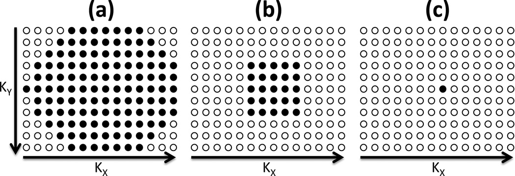
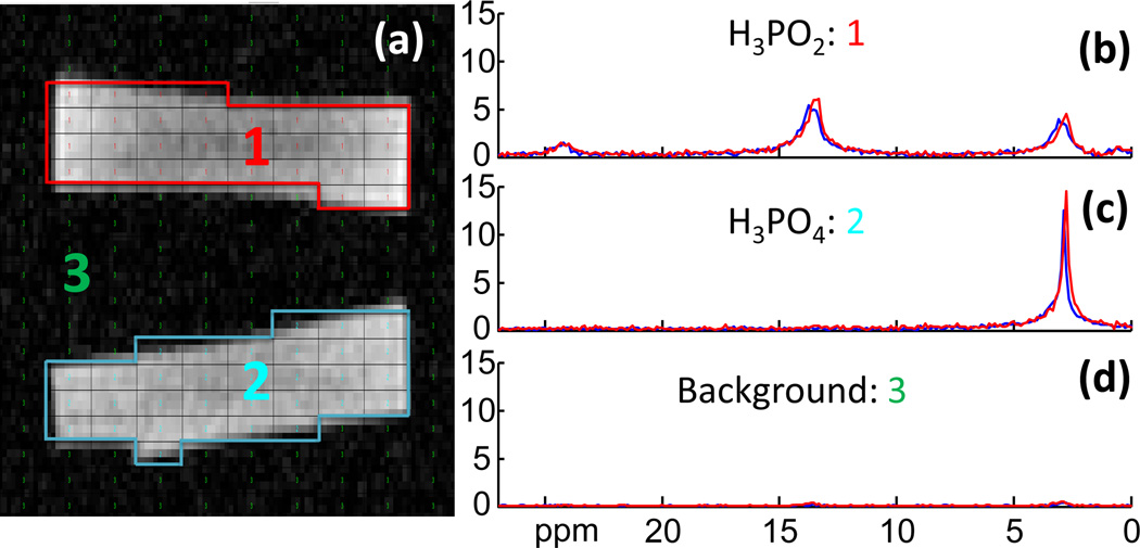
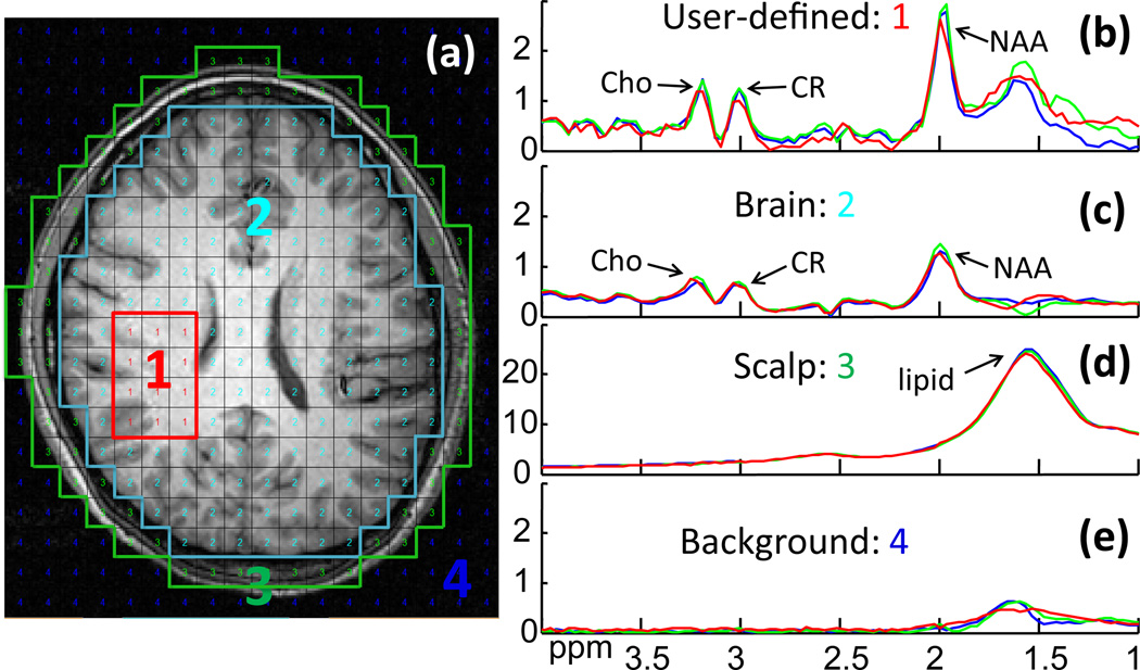
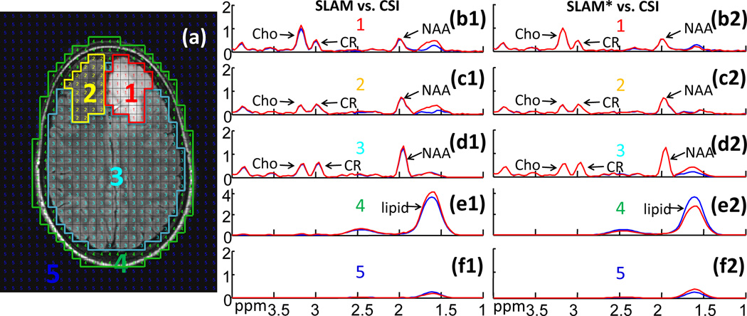
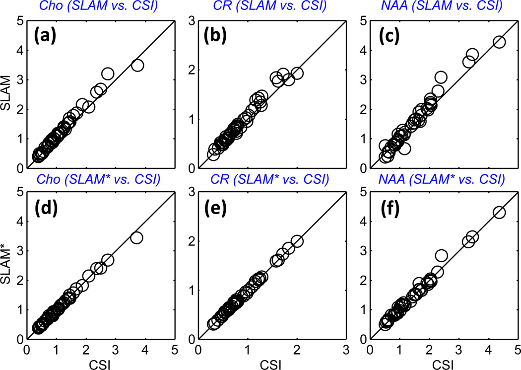
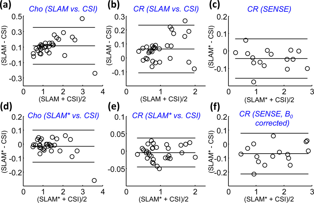
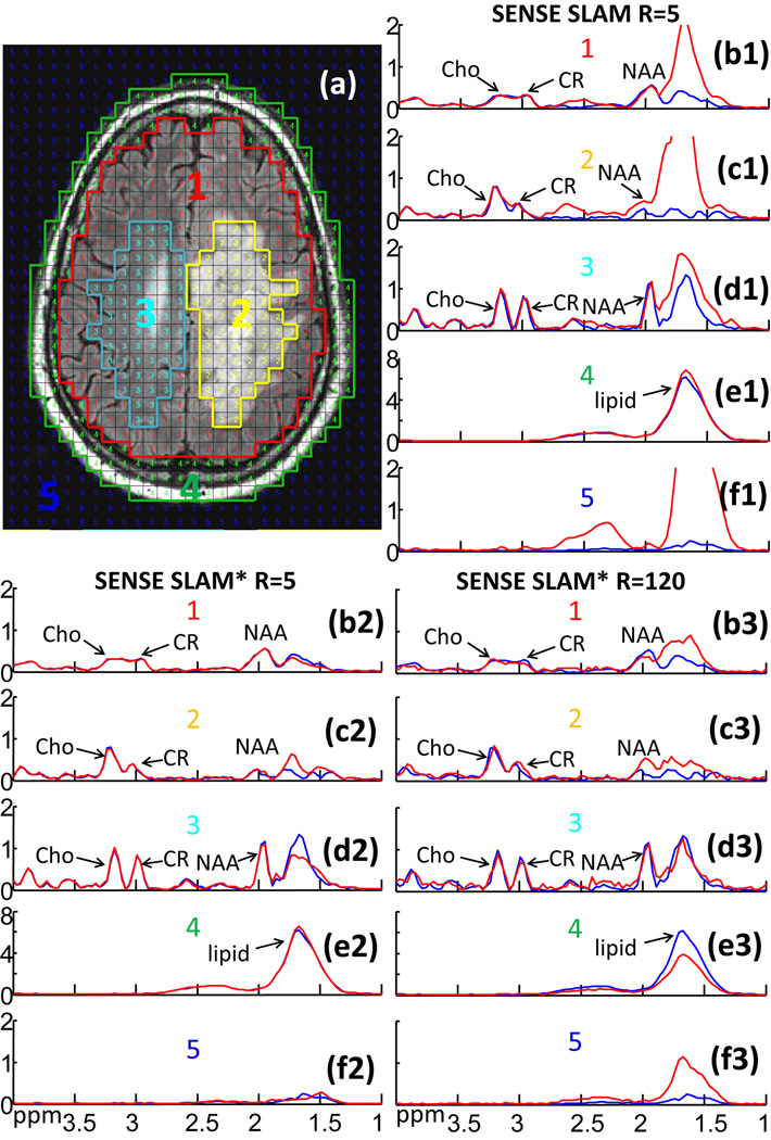
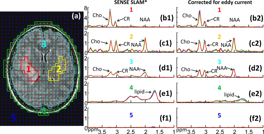
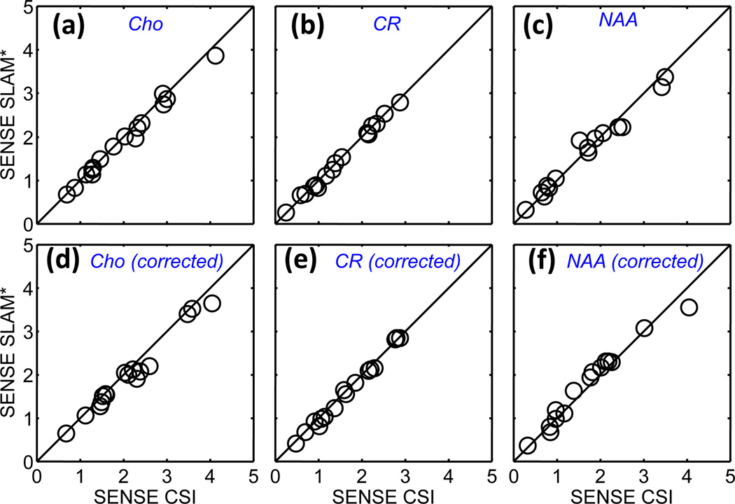
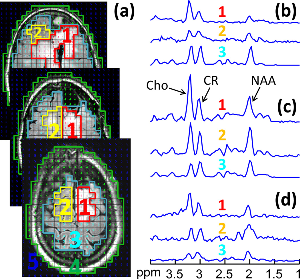
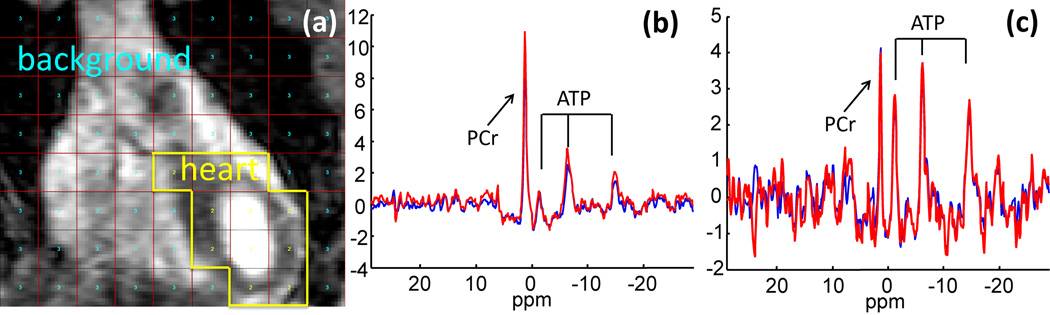
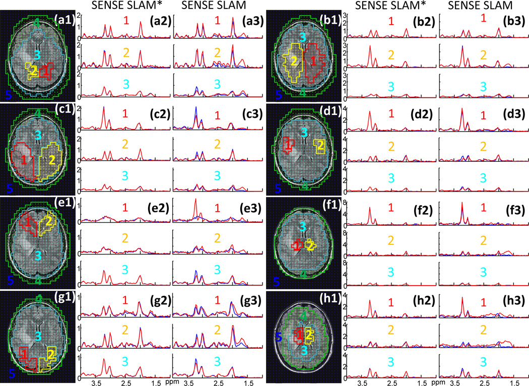
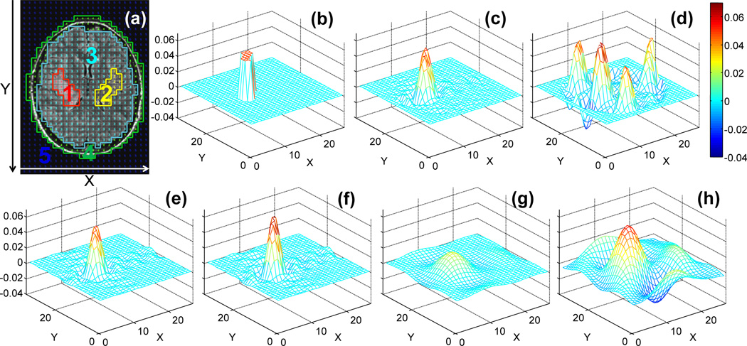
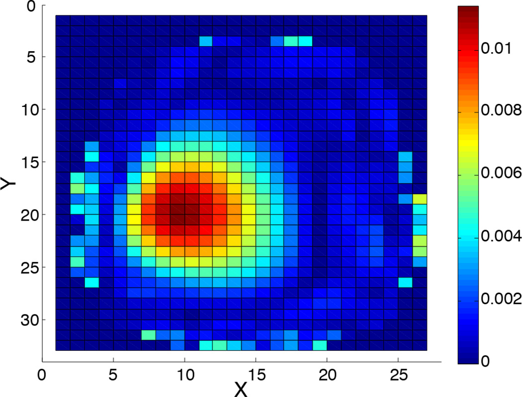
Noninvasive magnetic resonance spectroscopy (MRS) with chemical shift imaging (CSI) provides valuable metabolic information for research and clinical studies, but is often limited by long scan times. Recently, spectroscopy with linear algebraic modeling (SLAM) was shown to provide compartment-averaged spectra resolved in one spatial dimension with many-fold reductions in scan-time. This was achieved using a small subset of the CSI phase-encoding steps from central image k-space that maximized the signal-to-noise ratio. Here, SLAM is extended to two- and three-dimensions (2D, 3D). In addition, SLAM is combined with sensitivity-encoded (SENSE) parallel imaging techniques, enabling the replacement of even more CSI phase-encoding steps to further accelerate scan-speed. A modified SLAM reconstruction algorithm is introduced that significantly reduces the effects of signal nonuniformity within compartments. Finally, main-field inhomogeneity corrections are provided, analogous to CSI. These methods are all tested on brain proton MRS data from a total of 24 patients with brain tumors, and in a human cardiac phosphorus 3D SLAM study at 3T. Acceleration factors of up to 120-fold versus CSI are demonstrated, including speed-up factors of 5-fold relative to already-accelerated SENSE CSI. Brain metabolites are quantified in SLAM and SENSE SLAM spectra and found to be indistinguishable from CSI measures from the same compartments. The modified reconstruction algorithm demonstrated immunity to maladjusted segmentation and errors from signal heterogeneity in brain data. In conclusion, SLAM demonstrates the potential to supplant CSI in studies requiring compartment-average spectra or large volume coverage, by dramatically reducing scan-time while providing essentially the same quantitative results.

Keywords: Brain; Cancer; Chemical shift imaging (CSI); Heart; Localized spectroscopy; SLAM.

Figure 1

The k-space acquisition schemes for: (a) 11×14 SENSE CSI with corners omitted (120 steps); and SENSE SLAM/SLAM* acquisitions with further (b) 5-fold (25 steps total) and (c) 120-fold (1-step) acceleration factors, respectively. For simplicity, the 6-fold k-space undersampling afforded by SENSE, is omitted. Each filled circle denotes a k-space sample in the k_Y (or Y) and k_x (or X) directions.

Figure 2

Comparison of 3D proactive ³¹P SLAM spectra in a phantom. (a) Segmentation based on a co-registered phantom image. The CSI voxels are segmented into three compartments: 1, H₃PO₂; 2, H₃PO₄; 3, background. (b–d) Red SLAM spectra reconstructed from 20 phase encodes compared to the blue CSI compartmental average spectra reconstructed from 2000 phase encodes. The SLAM acceleration factor is R=100.

Figure 3

Retroactive and proactive SLAM in normal brain. (a) MRI of normal brain, overlaid with the CSI grid and segmented into four compartments post MRS acquisition: (1) user-defined area; (2) ‘rest of the brain’; (3) scalp; and (4) background. (b–d) 2D CSI (blue) and 2D SLAM spectra (red and green) acquired from the four compartments. The red SLAM spectra were acquired in a proactive scan using data 14 times faster than CSI. The green SLAM spectra were reconstructed retroactively from a subset of 1/14^th of the CSI data.

Figure 4

Comparison of SLAM and SLAM* brain spectra with CSI. (a) Image with co-registered CSI grid and segmented into five compartments: (1) tumor (low-grade astrocytoma); (2) contralateral brain; (3) ‘rest of the brain’; (4) scalp; and (5) background. Spectra (b1–f2) show the CSI spectra (blue) from the corresponding compartments, along with SLAM (b1–f1) and SLAM* (b2–f2) spectra (red) reconstructed from 1/6^th the CSI data for an acceleration factor R=6.

Figure 5

Quantitative comparison of SLAM and SLAM* with CSI data from the 16 patients. Cho, CR, and NAA levels (arbitrary units) as quantified in SLAM (a–c), and in SLAM* (d–f) spectra in tumor, contralateral brain and ‘rest of the brain’ compartments, as a function of those levels measured in the CSI spectra from the same compartments. The SLAM and SLAM* spectra were reconstructed from 1/6 of the 2D CSI data for an effective R=6. The correlation coefficients are R ≥ 0.98 for all cases.

Figure 6

Bland-Altman plots for Cho (a, c) and CR (b, e) measured by SLAM (a, b) and SLAM* (d,e), as compared to CSI. Parts (c) and (e) show Bland-Altman plots for CR measured by SENSE SLAM* as compared to SENSE CSI, without (c), and with (f) B₀ corrections.

Figure 7

2D retroactive SENSE SLAM and SENSE SLAM* results. (a) MRI showing segmentation of five compartments: (1) ‘rest of the brain’; (2) tumor (a glioblastoma); (3) contralateral brain; (4) scalp; and (5) background. Spectra (b1–f3) are from the corresponding compartments with SENSE CSI spectra in blue for comparison. SENSE SLAM spectra (b1–f1) and SENSE SLAM* spectra (b2–f2) in red, were reconstructed with 1/5^th of the SENSE CSI data, for an acceleration factor R=5. Spectra (b3-f3) were reconstructed with R=120 using SENSE SLAM*.

Figure 8

SENSE CSI and SLAM* spectra without and with eddy current corrections. (a) MRI depicting segmentation: (1) brain tumor; (2) contralateral brain; (3) ‘rest of the brain’; (4) scalp; and (5) background. Spectra (b1–f2) are from the corresponding compartments without (b1–f1) and with (b2–f2) eddy current correction. Blue spectra are SENSE CSI. The SENSE SLAM* spectra are reconstructed from 1/5^th of the CSI data set (green), or proactively in a separate scan with R=5 (red).

Figure 9

Quantitative comparison of SENSE SLAM* measures of Cho, CR, and NAA levels (arbitrary units) in tumor and contralateral brain with SENSE CSI measures from the same compartments, without (a–c) and with (d–f) eddy current corrections. The SENSE SLAM* spectra were reconstructed with 1/5^th of the CSI data for R = 5. Correlation coefficients are R ≥ 0.98 for all cases.

Figure 10

(a) Proactive SENSE SLAM* from the top three sections (separation, 17.6 mm) of a 5-slice data set, annotated to show: (1) tumor; (2) contralateral brain; (3) ‘rest of the brain’; (4) scalp; and (5) background compartments. (b–d) SENSE SLAM* spectra of the corresponding compartments in each of the three slices.

Figure 11

3D SLAM in a human ³¹P cardiac study. (a) Cardiac MRI showing segmented compartments: (1) chest; (2) heart; and (3) background. SLAM (red) and CSI (blue) spectra from (b) the chest and (c) the heart, with R = 7 and a 15 Hz exponential filter.

Figure 12

The effects of incorrect segmentation and inhomogeneity. (a1–h1) Brain MRI showing eight grossly maladjusted segmentations (Fig. 8a shows the correct segmentation). The corresponding SENSE SLAM* (a2–h2, red) and SENSE SLAM spectra (a3–h3, red) reconstructed from the maladjusted compartments are compared with the average SENSE CSI cspectra (blue) from the same compartments. For SENSE SLAM* and SENSE SLAM, R = 5 compared to SENSE CSI.

Figure 13

The computed tumor dSRF. (a) Brain MRI showing tumor segmentation(1, in red). The real part of dSRF is shown for the following reconstructions: (b) SENSE SLAM* (R=6 vs. SENSE CSI, without numeric regularization); (c) SENSE SLAM* (R = 6 vs. SENSE CSI, with numeric regularization and TSVD threshold ≤2% of the maximum); (d) SENSE SLAM (R=6 vs. SENSE CSI); (e) SLAM* (R=6 vs. CSI); (f) SLAM (R=6 vs. CSI); (g) SLAM* (R=36 vs. CSI); (h) SLAM (R=36 vs. CSI). Note that the dSRF is essentially not changed with or without the 2% TSVD in (d–h).

Figure 14

The computed dSRF for compartment #3 of Fig. 7 in the extreme case of a single phase-encode (intensity scale is arbitrary).

References

1. Hardy CJ, Weiss RG, Bottomley PA, Gerstenblith G. Altered myocardial high-energy phosphate metabolites in patients with dilated cardiomyopathy. American Heart Journal. 1991;122:795–801. - PubMed
1. Weiss RG, Bottomley PA, Hardy CJ, Gerstenblith G. Regional myocardial metabolism of high-energy phosphates during isometric exercise in patients with coronary artery disease. New England Journal of Medicine. 1990;323:1593–1600. - PubMed
1. Bottomley PA, Weiss RG. Non-invasive magnetic-resonance detection of creatine depletion in non-viable infarcted myocardium. The Lancet. 1998;351:714–718. - PubMed
1. Weiss RG, Gerstenblith G, Bottomley PA. ATP flux through creatine kinase in the normal, stressed, and failing human heart. Proceedings of the National Academy of Sciences of the United States of America. 2005;102:808–813. - PMC - PubMed
1. Smith CS, Bottomley PA, Schulman SP, Gerstenblith G, Weiss RG. Altered creatine kinase adenosine triphosphate kinetics in failing hypertrophied human myocardium. Circulation. 2006;114:1151–1158. - PMC - PubMed
Publication types