Posterior predictive Bayesian phylogenetic model selection

Abstract

We present two distinctly different posterior predictive approaches to Bayesian phylogenetic model selection and illustrate these methods using examples from green algal protein-coding cpDNA sequences and flowering plant rDNA sequences. The Gelfand-Ghosh (GG) approach allows dissection of an overall measure of model fit into components due to posterior predictive variance (GGp) and goodness-of-fit (GGg), which distinguishes this method from the posterior predictive P-value approach. The conditional predictive ordinate (CPO) method provides a site-specific measure of model fit useful for exploratory analyses and can be combined over sites yielding the log pseudomarginal likelihood (LPML) which is useful as an overall measure of model fit. CPO provides a useful cross-validation approach that is computationally efficient, requiring only a sample from the posterior distribution (no additional simulation is required). Both GG and CPO add new perspectives to Bayesian phylogenetic model selection based on the predictive abilities of models and complement the perspective provided by the marginal likelihood (including Bayes Factor comparisons) based solely on the fit of competing models to observed data.

Figure 1.

The notation y_i refers to a vector of length n_c that (assuming no missing data or ambiguities) has a single nonzero element (where n_c is the number of possible data patterns). This single nonzero element corresponds to the particular data pattern observed for site i and has value 1. The vector y₂ corresponding to site i = 2 is shown for illustration. The result (y_·) of summing y_i over all i = 1,2,··· ,n_s is also shown (where n_s is the number of sites).

Figure 2.

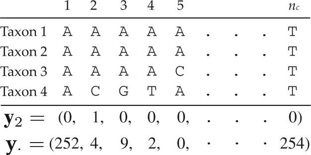
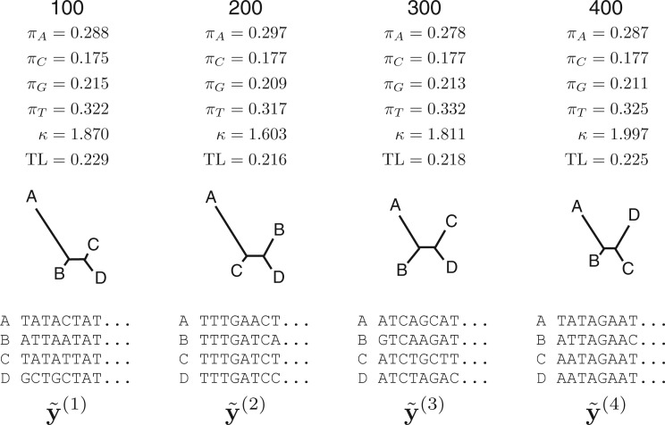
Generation of posterior predictive data sets under a HKY substitution model for a four-taxon problem. Numbers at the top represent the MCMC iteration at which a posterior sample was drawn, TL=tree length (sum of the five edge length parameters), κ =transition/transversion rate ratio, and π_A, π_C, π_G, π_T =nucleotide equilibrium relative frequencies. For each iteration, the sampled parameter values and tree are used to simulate one data set, the vector of pattern counts of which constitute .

Figure 3.

Comparison of prior models using the GG criterion for the gene psaB in the algae example data set. Solid line with squares: the mean number of distinct data patterns in posterior predictive data sets. Solid line with open circles: the overall GG measure (smallest is best). Dashed line with downward-pointing triangles: the goodness-of-fit component (GG_g) of the GG criterion. Dotted line with upward-pointing triangle: the variance component GG_p of the GG criterion. Trees shown below the plot are the last tree sampled for each of the eight analyses. The prior mean used for each analysis is 10^x, where x is the abscissa, except for the point labeled “hyper” in which the exponential prior mean was a hyperparameter in a hierarchical model.

Figure 4.

Plots of site-specific log(CPO) values for analyses of all four genes in the algae data set. a) Partitioned by gene (dotted vertical lines show gene boundaries). b) Partitioned by gene, but sorted by codon position, with 1st (left), 2nd position (center), and 3rd position (right) (dotted vertical lines show codon position boundaries). c) Partitioned by codon (dotted vertical lines show codon position boundaries).

Figure 5.

Plot of the log of the CPO ratio, equal to log(CPO3) −log(CPO5), where CPO5 is site-specific CPO estimated using the 5′ tree (on left), and CPO3 is site-specific CPO estimated using the 3′ tree (on right). Vertical dotted line separates 5′ end (left) from 3′ end (right) of the ribosomal protein gene rps11.

Figure 6.

Comparison of partition models for green algal protein-coding data. NONE is unpartitioned, GENE is partitioned by gene (four subsets), CODON is partitioned by codon position (three subsets), and BOTH is partitioned by both gene and codon position (12 subsets). Squares indicate GG, circles indicate SS, and triangles indicate LPML. Solid lines use scale on left; dotted line uses scale on right.

References

-
- Akaike H. A new look at statistical model identification. IEEE Trans. Automat. Contr. 1974;19:716–723.
- Arima S., Tardella L. Improved harmonic mean estimator for phylogenetic model evidence. J. Comput. Biol. 2012;19:418–438. - PubMed
- Bergthorsson U., Adams K.L., Thomason B., Palmer J.D. Widespread horizontal transfer of mitochondrial genes in flowering plants. Nature. 2003;424:197–201. - PubMed
- Bollback J. Bayesian model adequacy and choice in phylogenetics. Mol. Biol. Evol. 2002;19:1171–1180. - PubMed
Publication types
MeSH terms
Substances
Grants and funding
LinkOut - more resources
Full Text Sources
Other Literature Sources