Context-dependent computation by recurrent dynamics in prefrontal cortex

Abstract

Prefrontal cortex is thought to have a fundamental role in flexible, context-dependent behaviour, but the exact nature of the computations underlying this role remains largely unknown. In particular, individual prefrontal neurons often generate remarkably complex responses that defy deep understanding of their contribution to behaviour. Here we study prefrontal cortex activity in macaque monkeys trained to flexibly select and integrate noisy sensory inputs towards a choice. We find that the observed complexity and functional roles of single neurons are readily understood in the framework of a dynamical process unfolding at the level of the population. The population dynamics can be reproduced by a trained recurrent neural network, which suggests a previously unknown mechanism for selection and integration of task-relevant inputs. This mechanism indicates that selection and integration are two aspects of a single dynamical process unfolding within the same prefrontal circuits, and potentially provides a novel, general framework for understanding context-dependent computations.

Figure 1. Behavioral task and psychophysical performance

a, Task structure. Monkeys were instructed by a contextual cue to either discriminate the motion or the color of a random-dot stimulus, and indicate their choice with a saccade to one of two targets. Depending on context, monkeys were rewarded for choosing the target matching the prevalent direction of motion (motion context) or the prevalent color (color context) of the random-dots. Context was indicated by the shape and color of the fixation point; offset of the fixation point was the ‘go cue’, signaling the monkey to indicate its choice via the operant saccade. b, Stimulus set. The motion and color coherence of the dots was chosen randomly on each trial. We slightly varied the coherence values on each day, to equate performance across contexts and sessions (numbers in parentheses: average coherences (%) across sessions for monkey A). c-f, Psychophysical performance for monkey A in the motion (top) and color contexts (bottom), averaged over 80 recording sessions (163,187 trials). Performance is shown as a function of motion (left) or color (right) coherence in each behavioral context. The curves are fits of a behavioral model.

Figure 2. Dynamics of population responses in PFC

The average population response for a given condition and time is represented as a point in state space. Responses from correct trials only are shown from 100ms after dots onset (dots on, purple circle) to 100ms after dots offset (dots off) in 50ms steps, and are projected into the three-dimensional subspace capturing the variance due to the monkey’s choice (along the choice axis), and to the direction and strength of the motion (motion axis) and color (color axis) inputs. Units are arbitrary; components along the motion and color axes are enhanced relative to the choice axis (see scale bars in a,f). Conditions (see color bars) are defined based on context (motion context, top; color context, bottom), on the location of the chosen target (choice 1 vs. choice 2) and either on the direction and strength of the motion (gray colors) or the color input (blue colors). Here, choice 1 corresponds to the target in the response field of the recorded neurons. The direction of the color input does not refer to the color of the dots per se (red or green), but to whether the color points towards choice 1 or choice 2 (see Supplementary Information, section 6.4, for a detailed description of the conditions). a, Effect of choice and the relevant motion input in the motion context, projected onto the axes of choice and motion. b, Same data as in a, but rotated by 90° around the axis of choice to reveal the projection onto the axis of color. c, Same trials as in b, but re-sorted according to the direction and strength of the irrelevant color input. d-f, responses in the color context, analogous to a-c. Responses are averaged to show the effects of the relevant color (e,f) or the irrelevant motion input (d). For relevant inputs (a,b and e,f), correct choices occur only when the sensory stimulus points towards the chosen target (3 conditions per chosen target); for irrelevant inputs (c,d), however, the stimulus can point either towards or away from the chosen target on correct trials (6 conditions per chosen target).

Figure 3. Models of selective integration inconsistent with PFC responses

Schematic representation of population responses observed in PFC (a) and expected by several models of selective integration (b-d). The models differ from the PFC responses with respect to the relative directions and context dependence of the choice axis (red lines) and the inputs (thick gray arrows; only motion input shown). The relevant input is integrated as movement along the choice axis towards one of two choices (red crosses). A motion input towards choice 1 ‘pushes’ the responses along the direction of the gray arrow (towards choice 2: opposite direction). Same conditions as in Fig. 2a (motion context, top) and Fig. 2d (color context, bottom). As in Fig. 2a and d, a single two-dimensional subspace (which contains the choice axis and motion input) is used to represent responses from both contexts. a, Idealized schematic of the actual PFC trajectories shown in Fig. 2a,d. Both the choice axis and motion input are stable between contexts. The motion input pushes the population response away from the choice axis. b, Early selection model. When relevant (top), the motion input pushes the population response along the choice axis. When irrelevant (bottom), the motion input is filtered out before reaching PFC (no thick gray arrow) and thus exerts no effect on choice. All trajectories fall on top of each other in both contexts, but the rate of movement along the choice axis increases with motion strength only in the motion context (insets show enlarged trajectories distributed vertically for clarity). c, Context dependent input direction. Motion input direction varies between contexts, while the choice axis is stable. Inputs are not filtered out before PFC; rather they are selected based on their projection onto the choice axis. d, Context-dependent output direction. Similar selection mechanism to c, except that the choice axis varies between contexts, while the motion input is stable. The effects of the motion input on PFC responses in both monkeys (schematized in a) and the effects of the color input in monkey A are inconsistent with predictions of the three models in b-d (respectively, Fig. 2a,d; Extended Data Fig. 7a,d; Fig. 2f,c).

Figure 4. A neural network model of input selection and integration

PFC is modeled as a network of recurrently connected, nonlinear, rate neurons that receive independent motion, color, and contextual inputs. The network is fully recurrently connected, and each unit receives both motion and color inputs as well as two inputs that indicate context. At each time step, the sensory inputs are drawn from two normal distributions whose means correspond to the average strengths of the motion and color evidence on a given trial. The contextual inputs take one of two values (0 or 1), which instruct the network to discriminate either the motion or the color input. The network is read out by a single linear readout, corresponding to a weighted sum over the responses of all neurons (red arrows). We trained the network (with back-propagation) to make a binary choice, i.e. to generate an output of +1 at the end of the stimulus presentation if the relevant evidence pointed towards choice 1, or a −1 if it pointed towards choice 2. Before training, all synaptic strengths were randomly initialized.

Figure 5. Model dynamics and fixed points analysis

a-f, Dynamics of model population responses, same conventions as in Fig. 2. Responses are projected into the three-dimensional subspace spanned by the axes of choice, motion, and color (defined here based on the model synaptic weights, see Supplementary Information, section 7.6). Movement along the choice axis corresponds to integration of evidence, and the motion and color inputs deflect the trajectories along the corresponding input axes. Fixed points of the dynamics (red crosses) were computed separately for motion (a-c) and color contexts (d-f) in the absence of sensory inputs (see Supplementary Information, section 7.5). The fixed points are ‘marginally stable’ (i.e. one eigenvalue of the linearized dynamics is close to zero, while all others have strongly negative real parts; see Supplementary Information). The locally computed right zero-eigenvectors (red lines) point to the neighboring fixed points, which thus approximate a line attractor in each context. After the inputs are turned off (dots off, purple data points and lines) the responses relax back towards the line attractor. Each line attractor ends in two ‘stable’ attractors (i.e. all eigenvalues have strongly negative real parts, large crosses) corresponding to model outputs of +1 and −1 (i.e. choice 1 or 2).

Figure 6. Selection and integration by recurrent dynamics

a, Average model population response to short (1ms) pulses of motion (left) and color inputs (right) during motion (top) and color contexts (bottom). Motion or color inputs (solid lines) are initiated when the system is steady at one of the identified fixed points (red crosses), and subsequent relaxation back to the line attractor is simulated (dots: 3ms intervals) and averaged across fixed points. The size of the pulses approximately corresponds to the length of the scale bars in Fig. 5. Selection of the relevant input results from the context-dependent relaxation of the recurrent dynamics after the pulse, and is well approximated by the linearized dynamics around the fixed points (magenta lines). Responses are projected into the two-dimensional subspace spanned by the direction of the pulse and the locally computed line attractor (the right zero-eigenvector of the linearized dynamics). b, Explanation of how the same input pulse (left) leads to evidence integration in one context, but is ignored in the other (right). Relaxation towards the line attractor (small arrows) is always orthogonal to the context-dependent selection vector, and reverses the effects of the irrelevant pulse. c, Global arrangement of the line attractor (red) and selection vector (green) at each fixed point. Inputs are selected by the selection vector, which is orthogonal to the contextually irrelevant input (note input axes, right), and integrated along the line attractor.

Extended Data Figure 1. Recording locations and task-related patterns of population activity in PFC

a, Recording locations (red dots) in monkey A are shown on anatomical magnetic resonance images in imaging planes that were oriented perpendicularly to the direction of electrode penetrations. Electrodes were lowered through a grid (1mm spacing) positioned over the arcuate sulcus (AS). Recordings covered the entire depth of the AS and extended rostrally onto the prearcuate gyrus and cortex near and lateral to the principal sulcus. b-e, Representation of 4 task variables in the population response. Each multi-colored square corresponds to a recording location (red dots) in a. Within each square, each pixel corresponds to a unit recorded from that grid position, such that each square represents all the units recorded at the corresponding location. The color of a pixel indicates the de-noised regression coefficient of choice (b), motion coherence (c), color coherence (d), and context (e) for a given unit (color bars; gray: no units). These coefficients describe how much the trial-by-trial firing rate of a given unit depends on the task variables in b-e. The position of each unit within a square is arbitrary; we therefore sorted them according to the amplitude of the coefficient of choice, which accounts for the diagonal bands of color in b (top-left to bottom-right, high to low choice coefficient). The positions of the pixels established in b are maintained in c-e, so that one can compare the amplitude of the coefficient for each task variable for every unit recorded from monkey A. Each of the four panels can be interpreted as the pattern of population activity elicited by the corresponding task variable. The four task variables elicit very distinct patterns of activity and are thus separable at the level of the population. Importantly, the coefficients were de-noised with principal component analysis (see Suppl. Information, section 6.7) and can be estimated reliably from noisy neural responses (Extended Data Fig. 4i-l). Differences between activation patterns therefore reflect differences in the properties of the underlying units, not noise. f-j, Recording locations and task-related patterns of population activity for monkey F. Same conventions as in a-e. Recordings (f) covered the entire depth of the AS. The patterns of population activity elicited by a choice (g), by the motion evidence (h), and by context (j) are distinct, meaning that the representations of these task variables are separable at the level of the population. The representations of choice (g) and color (i), however, are not separable in monkey F, suggesting that color inputs are processed differently in the two monkeys (see main text).

Extended Data Figure 2. Psychophysical performance for monkey F and for the model

a-d, Psychophysical performance for monkey F, for motion (top) and color contexts (bottom), averaged over 60 recording sessions (123,550 trials). Performance is shown as a function of motion (left) or color (right) coherence in each behavioral context. As in Fig. 1c-f, coherence values along the horizontal axis correspond to the average low, intermediate and high motion coherence (a,c) and color coherence (b,d) computed over all behavioral trials. The curves are fits of a behavioral model (see Suppl. Information, section 4). e-h, ‘Psychophysical’ performance for the trained neural-network model (Figs. 4–6) averaged over a total of 14,400 trials (200 repetitions per condition). Choices were generated based on the output of the model at the end of the stimulus presentation—an output larger than zero corresponds to a choice to the left target (choice 1), and an output smaller than zero corresponds to a choice to the left target (choice 2). We simulated model responses to inputs with motion and color coherences of 0.03, 0.12, and 0.50. The variability in the input (i.e. the variance of the underlying Gaussian distribution) was chosen such that the performance of the model for the relevant sensory signal qualitatively matches the performance of the monkeys. As in Fig. 1c-f, performance is shown as a function of motion (left) or color (right) coherence in the motion (top) and color contexts (bottom). Curves are fits of a behavioral model (as in a-d and in Fig. 1c-f). In each behavioral context, the relevant sensory input affects the model’s choices (e, h), but the irrelevant input does not (f, g), reflecting successful context-dependent integration. In fact, the model output essentially corresponds to the bounded temporal integral of the relevant input (not shown) and is completely unaffected by the irrelevant input.

Extended Data Figure 3. Mixed representation of task variables in PFC

a-d, Example responses from 6 well-isolated single-units in monkey A. Each column shows average normalized responses on correct trials for one of the single-units. Responses are aligned to the onset of the random-dot stimulus, averaged with a 50ms sliding window, and sorted by one or more task-related variables (choice, motion coherence, color coherence, context). The green lines mark time intervals with significant effects of choice (a), motion coherence (b), color coherence (c), or context (d) as assessed by multi-variable, linear regression (regression coefficient different from zero, p<0.05). Linear regression and coefficient significance are computed over all trials (correct and incorrect, motion and color context; Supp. Information, section 6.3). The horizontal gray line corresponds to a normalized response equal to zero. a, Responses sorted by choice (solid: choice 1; dashed: choice 2) averaged over both contexts. b, Responses during motion context, sorted by choice and motion coherence (black to light-gray: high to low motion coherence). c, Responses during color context, sorted by choice and color coherence (blue to cyan: high to low color coherence). d, Responses sorted by choice and context (black: motion context; blue: color context). As is typical for PFC, the activity of the example units depends on many task variables, suggesting that they represent mixtures of the underlying task variables. e-f, De-noised regression coefficients for all units in monkey A (e) and monkey F (f). The data in Extended Data Fig. 1 are re-plotted here to directly compare the effects of different task variables (choice, motion, color, context) to each other. Each data point corresponds to a unit, and the position along the horizontal and vertical axes is the de-noised regression coefficient for the corresponding task variable. The horizontal and vertical lines in each panel intersect at the origin (0,0). Scale bars span the same range (0.1) in each panel. The different task variables are mixed at the level of individual units. While units modulated by only one of the task variables do occur in the population, they do not form distinct clusters but rather are part of a continuum that typically includes all possible combinations of selectivities. Significant correlations between coefficients are shown in red (p<0.05, Pearson’s correlation coefficient r).

Extended Data Figure 4. Targeted dimensionality reduction of population responses, and reliability of task-related axes and population trajectories

a, Fraction of variance explained by the first 20 principal components (PCs) of the responses in monkey A. PCs are computed on correct trials only, on condition-averaged responses. Conditions are defined based on choice, motion coherence, color coherence, and context. Each time point of the average response for a given condition contributes an ‘independent’ sample for the PC analysis, and variance is computed over conditions and times. b, Fraction of variance explained by the first 12 PCs. The total explainable variance (100%) is computed separately at each time, and reflects response differences across conditions. c, The four ‘task-related axes’ of choice, motion, color, and context expressed as linear combinations of the first 12 PCs. The four axes span a subspace containing the task-related variance in the population response (e.g. Fig. 2 and Extended Data Fig. 6) and are obtained by orthogonalizing the de-noised regression vectors for the corresponding task variables (see Suppl. information, section 6.7; de-noised regression coefficients are shown in Extended Data Figs. 1 and 3 e,f). The vertical axis in c corresponds to the projection of each axis onto a given PC (i.e. the contribution of that PC to each axis). All four axes project onto multiple PCs and thus the corresponding task variables are mixed at the level of single PCs. d, Fraction of variance explained by the task-related axes of choice, motion, color, and context (solid lines), as in b. The 4 axes explain a larger fraction of the variance than the PCs at many times but, unlike the PCs, they do not explain the variance common to all conditions that is due to the passage of time (not shown). A possible concern with our analysis is that the time courses of variance explained in d could be misleading if the task-related axes, which we estimated only at a single time for each variable, are in fact changing over time during the presentation of the random dots. Under this scenario, for example, the “humped” shape of the motion input (solid black trace) might reflect a changing ensemble code for motion rather than actual changes in the strength of the motion signal in the neural population. To control for this possibility, we also computed time-varying ‘task-related axes’ by estimating the axes of motion, color and context separately at each time throughout the 750ms dots presentation. The fractions of variance explained by the time-varying axes (dashed lines) and by the fixed axes (solid lines) have similar amplitudes and time courses. Thus the effects of the corresponding task variables (during the presentation of the random dots) are adequately captured by the subspace spanned by the fixed axes (see Suppl. Information, section 6.8). e-h, Same as a-d, for monkey F. As shown in Extended Data Figs. 1g,i and 3f (top-right panel) the de-noised regression coefficients of color and choice are strongly correlated. As a consequence, the axis of color explains only a small fraction of the variance in the population responses (h, blue; see main text). i-l, Reliability of task-related axes in monkey A. To determine to what extent variability (i.e., noise) in single unit responses affects the task-related axes of choice, motion, color, and context (e.g. Fig. 2 and Extended Data Fig. 6), we estimated each axis twice from two separate sets of trials (trial sets 1 and 2 in i-l). For each unit, we first assigned each trial to one of two subsets, and estimated de-noised regression coefficients for the task variables separately for the two subsets. We then obtained task-related axes by orthogonalizing the corresponding de-noised coefficients (see Suppl. Information, section 6.9). Here, the orthogonalized coefficients are computed both with (black) and without (gray) PCA based de-noising. The horizontal and vertical lines in each panel intersect at the origin (0,0). Scale bars span the same range (0.1) in each panel. Data points lying outside the specified horizontal or vertical plotting ranges are shown on the corresponding edges in each panel. i, Coefficients of choice. Each data point corresponds to the orthogonalized coefficient of choice for a given unit, computed from trials in set 1 (horizontal axis) or in set 2 (vertical axis). j-l, same as i for the orthogonalized coefficients of motion (j), color (k), and context (l). m-p, Orthogonalized regression coefficients for monkey F, as in i-l. Overall, after de-noising the orthogonalized coefficients are highly consistent across the two sets of trials. Therefore, the observed differences in the activation pattern elicited by different task variables (Extended Data Fig. 1) are not due to the noisiness of neural responses, but rather reflect differences in the properties of the underlying units. q-r, Reliability of population trajectories. To assess the reliability of the trajectories in Fig. 2, we estimated the task-related axes and the resulting population trajectories (same conventions as Fig. 2) twice from two separate sets of trials (as i-l, see Suppl. Information, section 6.9). As in the example trajectories shown in q (trial set 1) and r (trial set 2), we consistently obtained very similar trajectories across the two sets of trials. To quantify the similarity between the trajectories from the two sets, we used trajectories obtained from one set to predict the trajectories obtained from the other set (see Suppl. Information, section 6.9). On average across 20 randomly defined pairs of trial sets, in both monkeys the population responses from one set explain 94% of the total variance in the responses of the other set (95% for the example in q and r). These numbers provide a lower bound on the true reliability of trajectories in Fig. 2, with are based on twice as many trials as those in q and r.

Extended Data Figure 5. Population responses along individual task-related axes

a-e, Responses for monkey A. The average population responses on correct trials are re-plotted from Fig. 2, together with responses on a subset of incorrect trials (red curves). Here the responses are represented explicitly as a function of time (horizontal axis) and projected separately (vertical axes) onto the axes of choice (b), motion (c), color (d), and context (e). As in Fig. 2, correct trials are sorted based on context (motion: top sub-panels; color: bottom sub-panels; see key in a), on the direction of the sensory evidence (filled: towards choice 1; dashed: towards choice 2) and strength of the sensory evidence (black to light-gray: strongest to weakest motion; blue to cyan: strongest to weakest color), and based on choice (thick: choice 1; thin: choice 2). Incorrect trials (red curves) are shown for the lowest motion coherence (during motion context, top-left in b-e) and the lowest color coherence (during color context, bottom-right in b-e). Vertical scale bars correspond to 1 unit of normalized response, and the horizontal lines are drawn at the same level in all four sub-panels within b-e. a, Key to the condition-averages shown in each panel of b-e, as well as to the corresponding state-space panels in Fig. 2. b, Projections of the population response onto the choice axis. Responses along the choice axis represent integration of evidence in both contexts. c, Projection onto the motion axis. Responses along the motion axis represent the momentary motion evidence during both motion (top-left) and color contexts (bottom-left) (curves are parametrically ordered based on motion strength in both contexts), but not the color evidence (right, curves are not ordered based on color strength). d, Projection onto the color axis. Responses along the color axis represent the momentary color evidence in the motion (top-right) and color contexts (bottom-right) (ordered), but not the motion evidence (left, not ordered). e, Projection onto the context axis. Responses in the motion context (top, all curves above the horizontal line) and color context (bottom, all curves below the horizontal line) are separated along the context axis, which maintains a representation of context. f-i, Responses for monkey F, same conventions as in b-e. The responses in f-i are also shown as trajectories in Extended Data Fig. 7g-l. The drift along the choice axis in Extended Data Fig. 7g-l is reflected in the overall positive slopes in f.

Extended Data Figure 6. Effect of context on PFC dynamics

a-b, Responses from monkey A. Same conditions and conventions as in Fig. 2, but for activity projected into the two-dimensional subspace capturing the variance due to choice (along the choice axis) and context (context axis). Components along the choice axis are enhanced relative to the context axis (see scale bars). The population response contains a representation of context, which is reflected in the separation between trajectories in the motion and color contexts along the axis of context. The contextual signal is strongest early during the dots presentation. a, Effects of context (motion context vs. color context), choice (choice 1 vs. choice 2), and motion input (direction and coherence, gray colors). b, Same trials as in a, but averaged to show the effect of the color input (blue colors). c-d, Responses from monkey F, same conventions as in a-b. As in Extended Data Fig. 7a-f, we subtracted the across-condition average trajectory from each individual, raw trajectory (see Suppl. Information, section 6.10). The underlying raw population responses are shown in Extended Data Fig. 5f-i, and confirm that the representation of context is stable throughout the dots presentation time (Extended Data Fig. 5i).

Extended Data Figure 7. Dynamics of population responses in monkey F

a-f, Response trajectories in the subspace spanned by the task related axes of choice, motion, and color. Same conventions as in Fig. 2. Unlike in Fig. 2, here we subtracted the across-condition average trajectory from each individual, raw trajectory (see Suppl. Information, section 6.10). The raw trajectories are shown in panels g-l and the corresponding projections onto individual axes in Extended Data Fig. 5f-i. Three key features of the population responses are shared in monkey A (Fig. 2) and monkey F. First, movement along a single choice axis (a and f, red arrows) corresponds to integration of the relevant evidence in both contexts. Second, in both contexts the momentary motion evidence elicits responses along the axis of motion, which is substantially different from the axis of choice (a and d). Third, the motion evidence is strongly represented whether it is relevant (a) or irrelevant (d). Thus, the processing of motion inputs in both monkeys is inconsistent with current models of selection and integration (Fig. 3b-d). Unlike in monkey A, responses along the color axis in monkey F (f and c) reflect the momentary color evidence only weakly. The effects of color on the trajectories in monkey F resemble the responses expected by the early selection model (Fig. 3b). g-l, Raw population responses. Population trajectories were computed and are represented as in Fig. 2. The trajectories in a-f were obtained by subtracting the across-condition average from each individual trajectory shown above. Overall, the responses have a tendency to move towards the left along the choice axis. An analogous, though weaker, overall drift can also be observed in monkey A, and contributes to the asymmetry between trajectories on choice 1 and choice 2 trials (Fig. 2). Because choice 1 corresponds to the target in the response field of the recorded neurons (see Suppl. Information, section 6.2), the drift reflects a tendency of individual firing rates to increase throughout the stimulus presentation time. By the definition of choice 1 and choice 2, a similar but opposite drift has to occur in neurons whose response field overlaps with choice 2 (whose responses we did not record). In the framework of diffusion-to-bound models, such a drift can be interpreted as an urgency signal, which guarantees that the decision boundary is reached before the offset of the dots (Reddi and Carpenter, 2000; Churchland, Kiani and Shadlen, 2008).

Extended Data Figure 8. Simulations of models of selective integration inconsistent with PFC responses

We simulated population responses mimicking the observed PFC responses (a-c) and alternative responses expected based on the three models of context-dependent selection described in Fig. 3b-d (d-l) (see Suppl. Information, section 8). These simulations are based on a diffusion-to-bound model, unlike the simulations of the recurrent neural network models in Figs. 5,6 and in Extended Data Figs. 9 and 10e-s. Here, single neurons represent mixtures of three time-dependent task variables of a diffusion-to-bound model, namely the momentary motion and color evidence and the integrated relevant evidence. At the level of the population, these three task variables are represented along specific directions in state space (arrows in a,d,g,j; red, integrated evidence; black, momentary motion evidence; blue, momentary color evidence). The four simulations differ only with respect to the direction and context-dependence of the three task variables. We computed state space trajectories from the population responses using the targeted dimensionality reduction techniques discussed in the main text and in the Suppl. Information. The resulting simulated population responses reproduce the schematic population responses in Fig. 3. a-c, Simulated population responses mimicking the observed PFC responses (Fig. 2). a, Response trajectories in the 2d-subspace capturing the effects of choice and motion (left) or choice and color (right) in the motion (top) and color (bottom) contexts. Same conditions and conventions as in Fig 2a,c and Fig. 2d,f. The three task variables are represented along three orthogonal directions in state space (arrows). b, Regression coefficients of choice, motion, and color for all simulated units in the population. For each unit, coefficients were computed with linear regression on all simulated trials (top) or separately on trials from the motion or color context (bottom, context in parentheses). Scale bars represent arbitrary units. Numbers in the inset along each axis represent averages of the absolute value of the corresponding coefficients (±sem, in parentheses). c, Estimated strengths of the motion (top) and color (bottom) inputs during motion (black) and color (blue) contexts. Input strength is defined as the average of the absolute value of the corresponding regression coefficients. d-f, same as a-c, for simulated population responses expected from context-dependent early selection (Fig. 3b). When relevant, momentary motion (top) and color (bottom) evidence are represented along the same direction as integrated evidence (arrows in d). g-i, same as a-c, for simulated population responses expected from context-dependent input directions (Fig. 3c). Integrated evidence is represented along the same direction in both contexts (red arrows in g). The relevant momentary evidence (motion in the motion context, top; color in the color context, bottom) is aligned with the direction of integration, while the irrelevant momentary evidence is orthogonal to it (black and blue arrows in g). j-l, same as a-c, for simulated population responses expected from context-dependent output directions (Fig. 3d). The momentary motion and color evidence are represented along the same directions in both contexts (black and blue arrows in j). The direction of integration (red arrows in j) is aligned with the motion evidence in the motion context (top), and with the color evidence in the color context (bottom).

Extended Data Figure 9. Model population responses and validation of targeted dimensionality reduction

a-e, Model population responses along individual task-related axes, same conventions as in Extended Data Fig. 5. Here we defined the task-related axes directly based on the synaptic connectivity in the model (see Suppl. Information, section 7.6; and panels h-j), rather than using the approximate estimates based on the population response (as for the PFC data, e.g. Fig. 2). The same axes and the resulting projections underlie the trajectories in Fig. 5. The model integrates the contextually relevant evidence almost perfectly, and the responses along the choice axis (b) closely match the output of an appropriately tuned diffusion-to-bound model (not shown). Notably, near perfect integration is not a core feature of the proposed mechanism of context-dependent selection (see main text, and Extended Data Fig. 10). f-g, Effect of context on model dynamics, same conditions and conventions as in Extended Data Fig. 6. Network activity is projected onto the two-dimensional subspace capturing the variance due to choice (along the choice axis) and context (context axis). Same units on both axes (see scale bars). As in Fig. 5, fixed points of the dynamics (red crosses) and the associated right zero-eigenvectors (i.e. the local direction of the line attractor, red lines) were computed separately for motion (top) and color contexts (bottom) in the absence of sensory inputs. The line attractors computed in the two contexts, and the corresponding population trajectories, are separated along the context axis. f, Effects of context (motion context, color context), choice (choice 1, choice 2), and motion input (direction and coherence, gray colors) on the population trajectories. g, Same trials as in f, but re-sorted and averaged to show the effect of the color input (blue colors). The context axis is approximately orthogonal to the motion and color inputs, and thus the effects of motion and color on the population response (Fig. 5) are not revealed in the subspace spanned by the choice and context axes (f and g). h-j, Validation of targeted dimensionality reduction. To validate the dimensionality reduction approach used to analyze population responses in PFC (see Suppl. Information, sections 6.5–6.7), we estimated the regression vectors of choice, motion, color, and context from the simulated population responses (Fig. 5 and panels b-g) and compared them to the exactly known model dimensions that underlie the model dynamics (see definitions below). Here we estimated the regression vectors in three ways: by pooling responses from all model units and all trials (as in the PFC data, e.g. Fig. 2 and Extended Data Fig. 6), or separately from the motion- and color-relevant trials (contexts). Orthogonalization of the regression vectors yields the task-related axes of the subspace of interest (e.g. axes in Fig. 2). Most model dimensions (motion, color, and context inputs, and output) were defined by the corresponding synaptic weights after training. The line attractor, on the other hand, is the average direction of the right zero-eigenvector of the linearized dynamics around a fixed point, and was computed separately for the motion and color contexts. h, The three regression vectors of motion (black arrows), plotted in the subspace spanned by the choice axis (i.e. the regression vector of choice) and the motion axis (i.e. the component of the regression vector of motion orthogonal to the choice axis). In the color context, the motion regression vector closely approximates the actual motion input (black circle—the model dimension defined by synaptic weights). During the motion context, however, the motion regression vector has a strong component along the choice axis, reflecting the integration of motion evidence along that axis. The motion regression vector estimated from all trials corresponds to the average of the vectors from the two contexts; thus all three motion regression vectors lie in the same plane. i, The three regression vectors of color (blue arrows) plotted in the subspace spanned by the choice and color axes, analogous to h. The color regression vector closely approximates the actual color input (blue circle) in the motion context, but has a strong component along the choice axis in the color context. Components along the motion (h) and color (i) axes are scaled by a factor of 2 relative to those along the choice axis. j, Dot products (color bar) between the regression vectors (horizontal axis) and the actual model dimensions (vertical axis), computed after setting all norms to 1. The choice regression vector closely approximates the direction of the line attractor in both contexts (squares labeled ‘1’). As shown also in h and i, the input regression vectors approximate the model inputs (defined by their synaptic weights) when the corresponding inputs are irrelevant (squares 2 and 4, motion and color), while they approximate the line attractor when relevant (squares 3 and 5). Thus the motion input is mostly contained in the plane spanned by the choice and motion axes (h), and the color input is mostly contained in the plane spanned by the choice and color axes (i). Finally, the single context regression vector is aligned with both context inputs (squares 6), and closely approximates the difference between the two (not shown).

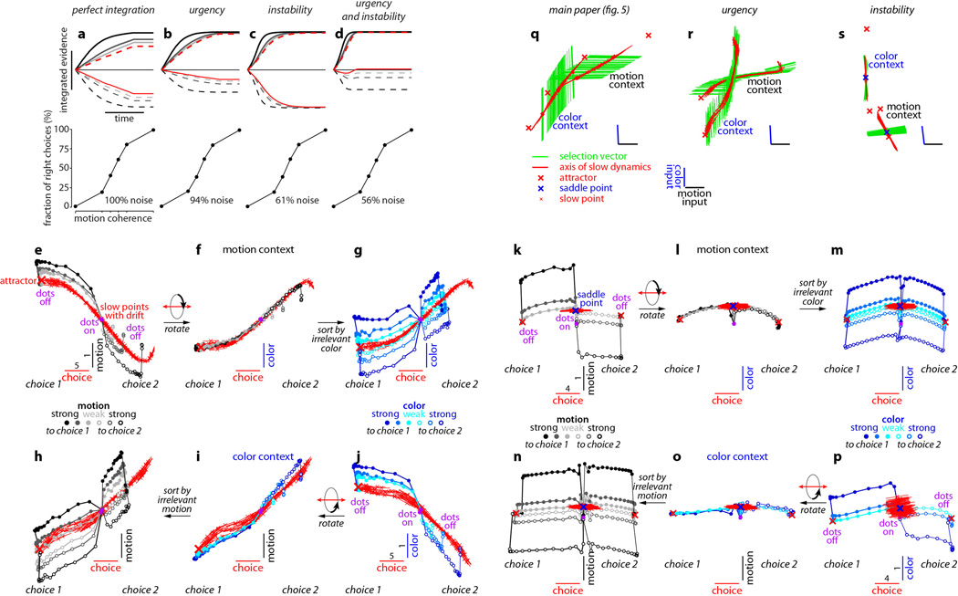
Extended Data Figure 10. Urgency and instability in the integration process

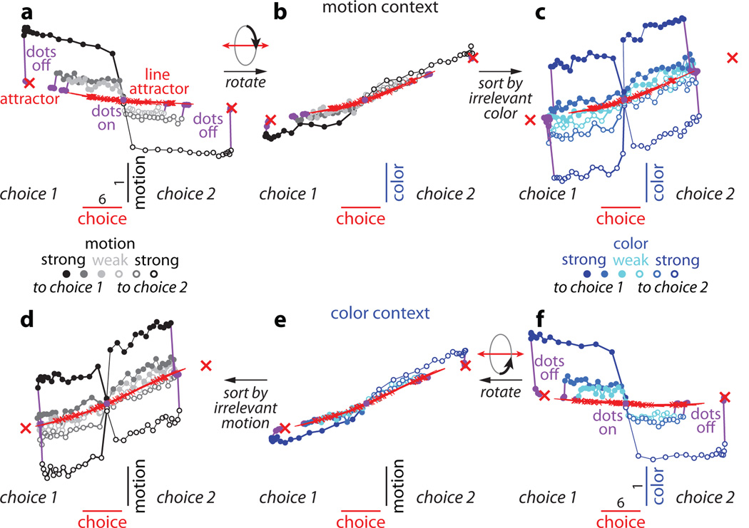
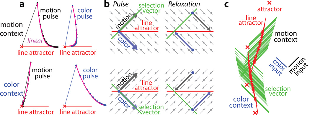
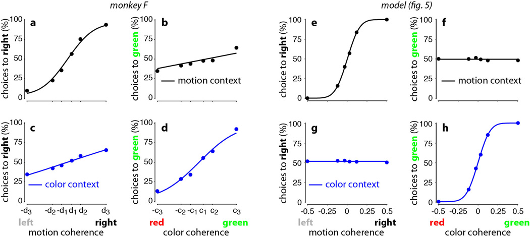
a-d, Choice predictive neural activity (top) and psychometric curves (bottom) predicted by several variants of the standard diffusion-to-bound model (see Suppl. information, section 7.7). a, Standard diffusion-to-bound model. Noisy momentary evidence is integrated over time until one of two bounds (+1 or −1; choice 1 or choice 2) is reached. The momentary evidence at each time point is drawn from a Gaussian distribution whose mean corresponds to the coherence of the input, and whose fixed variance is adjusted in each model to achieve the same overall performance (i.e. similar psychometric curves, bottom panels). Coherences are 6, 18, and 50% (the average color coherences in monkey A, Fig. 1b). Average integrated evidence (neural firing rates, arbitrary units) is shown on choice 1 and choice 2 trials (thick vs. thin) for evidence pointing towards choice 1 or choice 2 (solid vs. dashed), on correct trials for all coherences (light gray to black, low to high coherence), and incorrect trials for the lowest coherence (red). The integrated evidence is analogous to the projection of the population response onto the choice axis (e.g. Extended Data Fig. 5b, top-left and bottom-right). b, Urgency model. Here the choice is determined by a race between two diffusion processes (typically corresponding to two hemispheres), one with bound at +1, the other with bound at −1. The diffusion in each process is subject to a constant drift towards the corresponding bound, in addition to the drift provided by the momentary evidence. The input-independent drift implements an ‘urgency’ signal, which guarantees that one of the bounds is reached within a short time. Only the integrated evidence from one of the diffusion processes is shown. The three ‘choice 1’ curves are compressed (in contrast to a) because the urgency signal causes the bound to be reached, and integration toward choice 1 to cease, more quickly than in a. In contrast, the ‘choice 2’ curves are not compressed since the diffusion process that accumulates evidence toward choice 1 never approaches a bound on these trials. c, Same as a, but here the diffusion process is subject to a drift away from the starting point (0) towards the closest bound (+1 or −1). The strength of the drift is proportional to the distance from the starting point, and creates an ‘instability’ at the starting point. d, Same as b, with an instability in the integration as in c for both diffusion processes. The asymmetry between choice 1 and choice 2 curves in b and d resembles the asymmetry in the corresponding PFC curves (Extended Data Figs. 5b,f, upper left). e-j, Neural network model with urgency. This model is based on a similar architecture as the model in Fig. 4. Unlike the neural network in Fig. 4, which was trained solely based on the model output on the last time bin of the trial, here the network is trained based on the output it produces throughout the entire input presentation. The network was trained to reproduce the integrated evidence (i.e. the decision variable) for one of the two diffusion processes (i.e. one of the two ‘hemispheres’) in a diffusion-to-bound model with urgency (b, see Suppl. Information, section 7.7). Similar conventions as in Fig. 5. The urgency signal is controlled by an additional binary input into the network. Here, the urgency and sensory inputs are turned off as soon as a bound is reached. The network generates only a single, stable fixed point in each context, corresponding to the decision boundary (large red cross). The model also implements a series of points of relatively slow dynamics (small red crosses) approximately lying on a single curve. The axes of slow dynamics at these slow points (red lines) are locally aligned. Notably, responses at these slow points have a strong tendency to drift towards the single, stable fixed point (the decision boundary), and thus the curve of slow points does not correspond to an approximate line attractor. This drift implements the urgency signal and causes an asymmetry in the trajectories, which converge on a single point for choice 1, but have endpoints that are parametrically ordered by coherence along the choice axis for choice 2. As discussed below (panel r), this model relies on the same mechanism of selection as the original model (Fig. 5, see main text). k-p, Neural network model with instability. Trajectories show simulated population responses for a model (same architecture as in Fig. 4) that was trained to solve the context-dependent task (Fig. 1) only on high-coherence stimuli and in the absence of internal noise (see Suppl. Information, section 7.7). Same conventions as in Fig. 5. In the absence of noise, prolonged integration of evidence is not necessary for accurate performance on the task. As a consequence, the model implements a saddle point (blue cross) instead of an approximate line attractor. Points of slow dynamics (small red crosses, obscured by the red lines) occur only close to the saddle point. The right-zero-eigenvectors of the linearized dynamics around these slow points (red lines) correspond to the directions of slowest dynamics, and determine the direction of the axis of choice. When displaced from the saddle point, the responses quickly drift towards one of the two stable attractors (large red crosses) corresponding to the choices. For a given choice, trajectories for all coherences therefore end in the same location along the choice axis, in contrast to the responses in the original model (Fig. 5). Despite these differences, the original model (Fig. 5) and the network model with instability (k-p) rely on a common mechanism of context-dependent selection (see panel s). q-s, Dynamical features (key, bottom) underlying input selection and choice in three related neural network models. All models are based on a common architecture (Fig. 4) but are the result of different training procedures. q, Dynamical features of the model described in the main paper (Figs. 5–6), re-plotted from Fig. 6c. r, The urgency model (e-j). s, The instability model (k-p). In all models, the developing choice is implemented as more or less gradual movement along an axis of slow dynamics (specified by the locally computed right-eigenvectors associated with the near-zero eigenvalue of the linearized dynamics, red lines). The inputs are selected, i.e. result in movement along the axis of slow dynamics, depending on their projection onto the selection vector (the locally computed left-eigenvectors associated with the near-zero eigenvalue). In this sense, the three models implement the same mechanisms of context-dependent selection and choice.

References

1. Fuster JM. The prefrontal cortex. 4th edn. Academic Press; 2008.
1. Miller EK, Cohen JD. An integrative theory of prefrontal cortex function. Annu Rev Neurosci. 2001;24:167–202. - PubMed
1. Desimone R, Duncan J. Neural mechanisms of selective visual attention. Annu Rev Neurosci. 1995;18:193–222. - PubMed
1. Schroeder CE, Lakatos P. Low-frequency neuronal oscillations as instruments of sensory selection. Trends Neurosci. 2009;32:9–18. - PMC - PubMed
1. Noudoost B, Chang MH, Steinmetz NA, Moore T. Top-down control of visual attention. Curr Opin Neurobiol. 2010;20:183–190. - PMC - PubMed
Publication types