Failure mode analysis of silicon-based intracortical microelectrode arrays in non-human primates

Abstract

Objective: Brain-computer interfaces (BCIs) using chronically implanted intracortical microelectrode arrays (MEAs) have the potential to restore lost function to people with disabilities if they work reliably for years. Current sensors fail to provide reliably useful signals over extended periods of time for reasons that are not clear. This study reports a comprehensive retrospective analysis from a large set of implants of a single type of intracortical MEA in a single species, with a common set of measures in order to evaluate failure modes.

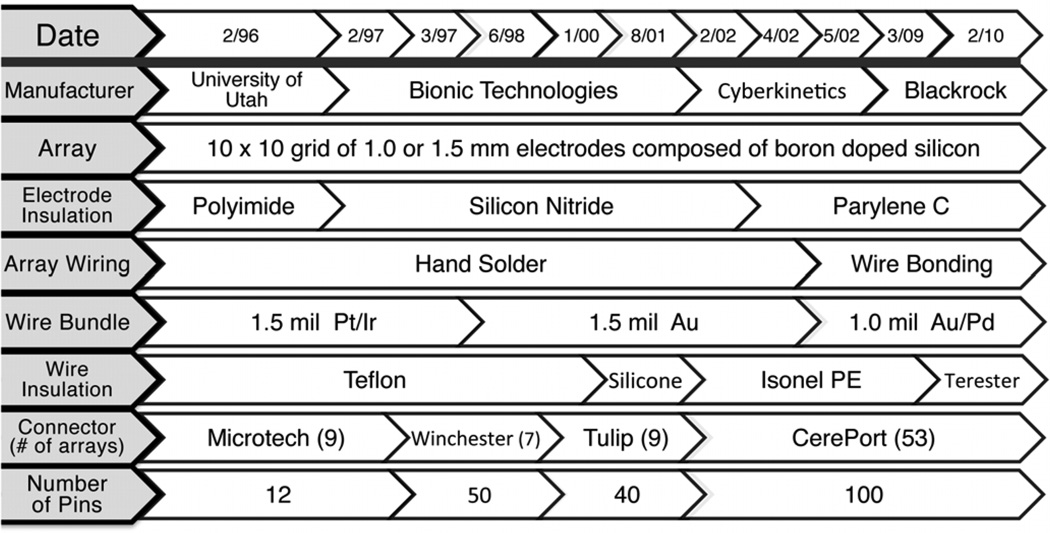
Approach: Since 1996, 78 silicon MEAs were implanted in 27 monkeys (Macaca mulatta). We used two approaches to find reasons for sensor failure. First, we classified the time course leading up to complete recording failure as acute (abrupt) or chronic (progressive). Second, we evaluated the quality of electrode recordings over time based on signal features and electrode impedance. Failure modes were divided into four categories: biological, material, mechanical, and unknown.

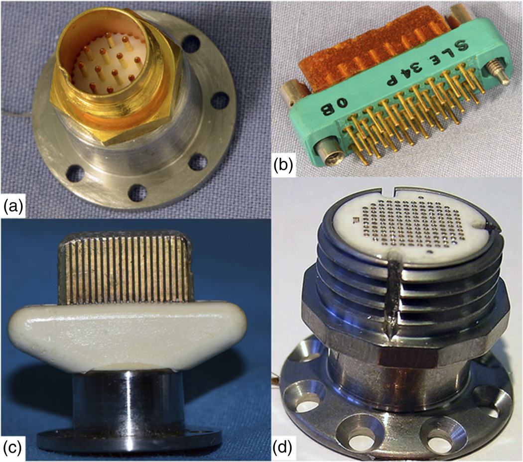
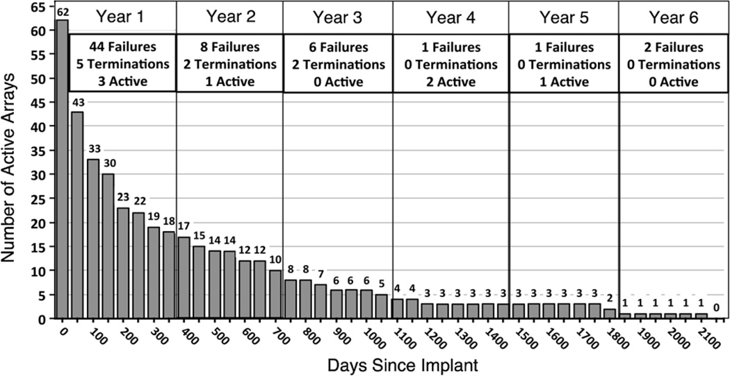
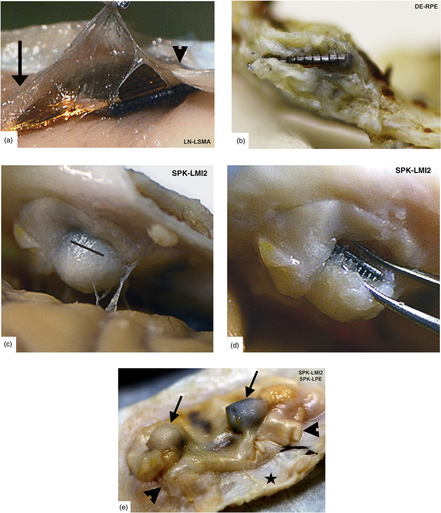
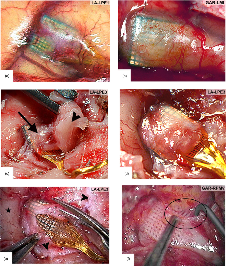
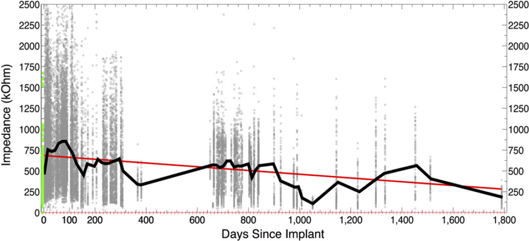
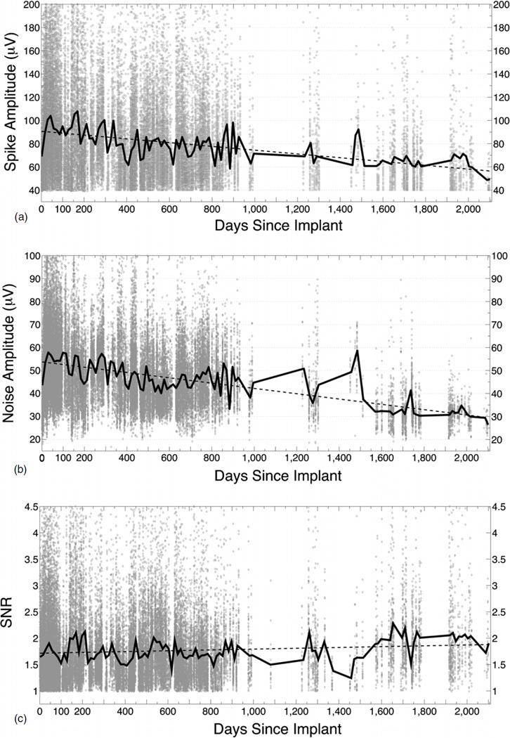
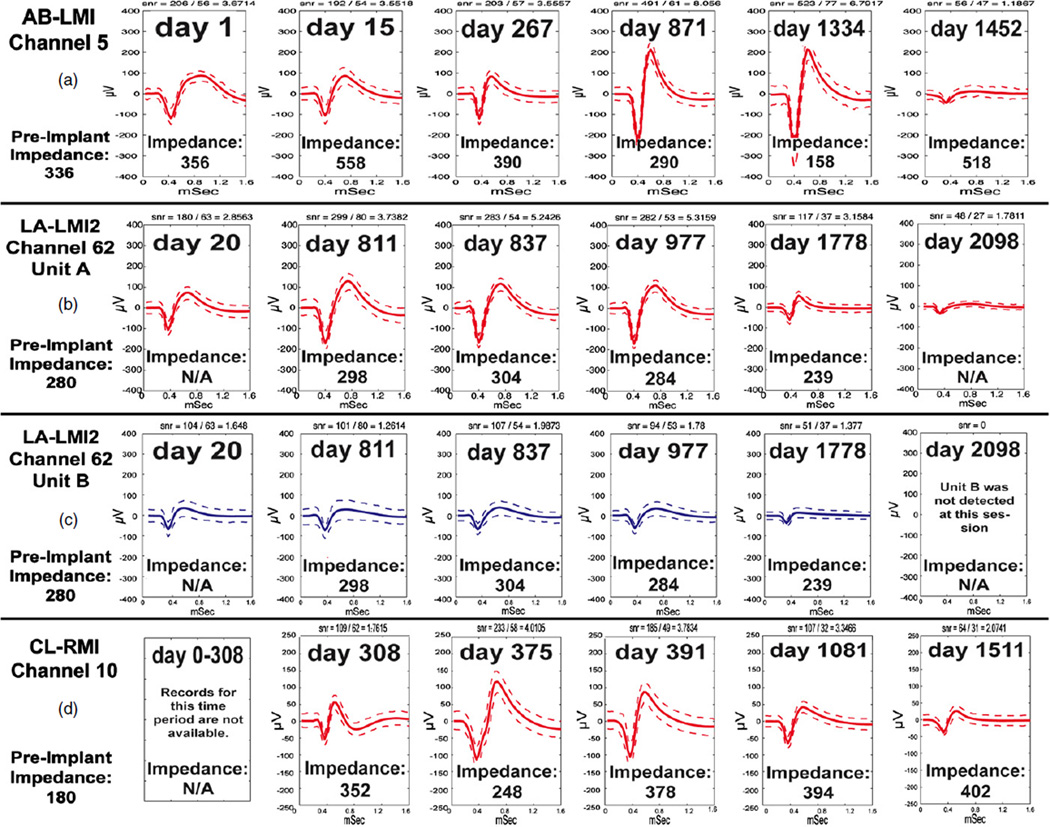
Main results: Recording duration ranged from 0 to 2104 days (5.75 years), with a mean of 387 days and a median of 182 days (n = 78). Sixty-two arrays failed completely with a mean time to failure of 332 days (median = 133 days) while nine array experiments were electively terminated for experimental reasons (mean = 486 days). Seven remained active at the close of this study (mean = 753 days). Most failures (56%) occurred within a year of implantation, with acute mechanical failures the most common class (48%), largely because of connector issues (83%). Among grossly observable biological failures (24%), a progressive meningeal reaction that separated the array from the parenchyma was most prevalent (14.5%). In the absence of acute interruptions, electrode recordings showed a slow progressive decline in spike amplitude, noise amplitude, and number of viable channels that predicts complete signal loss by about eight years. Impedance measurements showed systematic early increases, which did not appear to affect recording quality, followed by a slow decline over years. The combination of slowly falling impedance and signal quality in these arrays indicates that insulating material failure is the most significant factor.

Significance: This is the first long-term failure mode analysis of an emerging BCI technology in a large series of non-human primates. The classification system introduced here may be used to standardize how neuroprosthetic failure modes are evaluated. The results demonstrate the potential for these arrays to record for many years, but achieving reliable sensors will require replacing connectors with implantable wireless systems, controlling the meningeal reaction, and improving insulation materials. These results will focus future research in order to create clinical neuroprosthetic sensors, as well as valuable research tools, that are able to safely provide reliable neural signals for over a decade.

Figure 1

Silicon MEA with CerePort connector. Left: Scanning electron micrograph of a 100-electrode array. Right: Bundle of 96 wires running to Ti pedestal connector, which is secured to the skull using titanium screws. The connector pads mate to a spring-pin loaded ‘patient cable’ connector that screws onto the pedestal and delivers signals to a preamplifier (See Cerebus^® Neural Signal Processing System: User’s Manual, revision 13.0). The implant has two common signal reference wires, placed in the recording field (usually subdural).

Figure 2

Developmental process of the ‘Utah’ array. This table summarizes the approximate dates at which each design feature was implemented beginning with arrays fabricated in the Normann Laboratory at the University of Utah, then later by commercial entities (Bionic, Cyberkinetics, and Blackrock). Note that the form of the array has remained the same, but insulation, fabrication methods, wire bundle composition, connector type and number of possible connections have been modified over the years.

Figure 3

Types of connectors used across this study arranged according to their history of use. (a) Initial Microtech connector with 12 pins. (b) Winchester style connector with 34 pins. (c) Tulip connector with 40 pins. (d) Current CerePort connector with 100 functional contact pads.

Figure 4

Major failure modes of MEAs. (a) Ideal placement in cortical tissue, about 1 (or 1.5) mm into the cortex. A thin layer of arachnoid overgrowth encases the platform that sits on the pia-arachnoid surface and helps to stabilize the array. (b) Biological failures: bleeding, cell death, hardware infection, meningitis, gliosis, or meningeal encapsulation and extrusion. Macrophages originating in the subarachnoid space may mediate the encapsulation response. (c) Material failures: broken electrode tips, insulation leakage, or parylene cracks and delamination. Note that the latter three would lead to lower impedances and spike amplitudes due to shunting. (d) Mechanical failures: wire bundle damage, connector damage, and mechanical removal. A dural stitch is shown as one possible source of tethering that results in electrodes being pulled out of the brain.

Figure 5

Array time to failure. All array durations are aligned to the time of implantation. This chart shows how many of the failed arrays (n = 62) remained active at 50-day intervals from implantation. A yearly summary of all array (n = 78) outcomes is presented in the boxes along the top of the chart. The yearly summaries account for the arrays that were electively terminated (n = 9) or remained active (n = 7) at the close of this study.

Figure 6

Failures by mode. (a) This chart shows the number of arrays that failed by each failure mode category. Note that acute mechanical failures were most common. (b) This chart shows the mean time to failure for each class of failure modes. Error bars indicate the sem. Note that the chronic unknown failure category had the longest mean time to failure.

Figure 7

Encapsulated arrays–gross specimens. All of our arrays showed grossly visible encapsulation, however the extent of encapsulation varied greatly. (a) Thin tissue capsule with arachnoid appearance at 37 days post-implant. This tissue can be seen merging with normal arachnoid to the left (arrow) and normal dura to the right (arrowhead). (b) Dense fibrous tissue encapsulation at 761 days post-implant. The array is intradural in this photo. (c) Complete encapsulation by day 853. The capsule was cut open (black line) in order to visualize the array seen in (d). (e) Two arrays with varying degrees of thick encapsulation tissue (arrows) under each array at 853 days (viewed from below). A Teflon layer (Gore^® Preclude^® Dura Substitute, WL Gore and Associates, Flagstaff, AZ) was placed above the array and below the dura during implantation to prevent encapsulation. This photo indicates that subdural Teflon does not prevent encapsulation and extrusion, as the Teflon sheet was also encapsulated. Arrowheads indicate its location between the fibrous tissue capsule and the adjacent dura (black star). (Array names reflect monkey name and implant location).

Figure 8

Encapsulated arrays –intra-operative specimens. (a) Thin arachnoid encapsulation tissue with prominent neovascularization over the top of an array at 264 days post-implant. The dura was reflected with minimal adherence to this tissue. (b) An array explanted at 765 days post-implant with a slightly thicker arachnoid encapsulation, but no dural adhesions. (c) Surgical removal of dura (arrowhead) adherent to the arachnoid encapsulation (arrow) of an array at 1051 days post-implant. (d) The arachnoid encapsulation after dura has been removed. Note how the cortex is depressed at the implant site. (e) Microsurgical dissection of the same arachnoid capsule from (d) as seen through an operating microscope. Normal cortex (covered with normal arachnoid) is indicated by the black star. Dura is indicated at the borders by arrowheads. (f) After removing the array, a thickened arachnoid layer is observed below the array with a grid-like pattern caused by the individual electrodes. The picture shown, however, is from a different monkey explanted at 554 days with nearly identical findings. This photo shows that as the floor of the capsule is gently pulled aside, additional meningeal encapsulation tissue can be seen along the electrode tracts, diving down into the cortex (black circle). (Array names reflect monkey name and implant location.)

Figure 9

Impedance over time. Every 1 kHz impedance value (<2500 kΩ) for 26 arrays across 305 sessions is shown as a scatter plot (background dots, n= 29 280). The green points represent all pre-implant impedances as reported by the manufacturer. The black line plots the mean impedance value across all arrays per 14-day bin. Red ticks along the x-axis indicate bin margins. The red line is the linear regression fit (y = −0.23x + 6.9e + 002).

Figure 10

Selected impedance trends. (a) Three arrays with abundant short- and long-term impedance data. The recording sessions were divided into pre-implant values, immediate post-implant values (0–10 days), 3-month post-implant values (10–100 days), and long-term values (200–1000 days). The mean impedance at each session for each array was calculated and the mean across all sessions (per epoch) for each array was plotted. Impedances rise about three-fold in the first ten days after implantation, plateau over the next 3–4 months, then fall steadily over time. The cause of these changes may be independent and are not revealed by this plot. (b) Seven arrays with abundant impedance data over the first year since implant. The mean impedance for each array at each session is plotted. These results demonstrate that the global trends seen across all arrays reflect individual trends as well. Impedances rise dramatically in the first 10 days after implantation, plateau for the next 100 days, then drop. The rate of decay seems to slow after 200 days. (Array names reflect monkey name and implant location.)

Figure 11

Viable channels over time. The number of viable channels per array at each recording session for 47 CerePort arrays is shown as a scatter plot (colored dots). A different color and/or shape marker represents each array (see legend). The black line is the mean value across all arrays per 14-day bin. Red ticks along the x-axis indicate bin margins. The red line shows the linear regression (y = −0.016x + 59). The total number of data points (recording sessions) is n = 1073. (Array names reflect monkey name and implant location.)

Figure 12

Signal quality over time. (a) Spike amplitude of viable channels over time. The spike amplitude (PTP) per viable channel per array at each recording session for 47 arrays is shown as a scatter plot (background dots, n = 103 008). The black line is the mean value across all arrays per 14-day bin. The dotted line is the linear regression (y = −0.017x + 91). Note that spike amplitude is not predicted by the impedance (figure 9). (b) Noise amplitude of viable channels over time. The noise amplitude per channel per array at each recording session for 47 arrays is shown as a scatter plot (background dots, n = 103 008). The black line is the mean value across all arrays per 14-day bin. The dotted line is the linear regression (y = −0.012x + 54). Note that the noise amplitude drops at a similar rate as the spike amplitude. (c) SNR of viable channels over time. The SNR per channel per array at each recording session for 47 arrays is shown as a scatter plot (background dots, n = 103 008). The black line is the mean value across all arrays per 14-day bin. The dotted line is the linear regression (y = 7.8e–005x + 1.7).

Figure 13

Rates of signal decay. This graph overlaps linear regression models for impedance and spike amplitude (PTP), in order to compare their intercepts (note that slopes cannot be compared because axes are different). Critical values (empirically derived) where the system has failed are plotted as dashed lines. Thus, mean impedance values that degrade to <50 kΩ suggest that signals are largely shunted to ground; spikes with amplitudes <40 µV are effectively impossible to separate from background noise. The different y intercepts could suggest multiple, interacting failure modes but the data suggest that the technology could function for up to eight years.

Figure 14

Correlation between spike amplitude and impedance. All recording sessions with concurrent impedance measurements and spike amplitudes were compiled (n = 104). The data was then divided into four groups: (a) immediate post-implant values (0–10 days), (b) 3-month post-implant values (10–100 days), (c) long-term values (365 + days), and (d) all values. For each data subset, a correlation coefficient was calculated. The total number of data points is 9919. A very small, significant, positive correlation was found at all time points except for the long-term, where a small, but significant, negative correlation was found. These results suggest that multiple factors beyond impedance determine signal quality.

Figure 15

Recording quality of selected channels over time. (a) A channel showing spike recordings where shape and amplitude vary in size at different times, without a clear trend in any direction. (b) One of two units on a selected channel from the longest lasting array. Spikes were evident and impedances were stable for over four years. (c) A second, smaller unit on the same channel from (b). Note different trends in amplitude changes, except that the last recordings in every case had the smallest waveforms. (d) A third long-term array, showing a decline in signal amplitude for this channel despite stable impedances. (Array names reflect monkey name and implant location.)

References

1. Bansal AK, Truccolo W, Vargas-Irwin CE, Donoghue JP. Decoding 3D reach and grasp from hybrid signals in motor and premotor cortices: spikes, multiunit activity, and local field potentials. J. Neurophysiol. 2012;107:1337–1355. - PMC - PubMed
1. Biran R, Martin DC, Tresco PA. Neuronal cell loss accompanies the brain tissue response to chronically implanted silicon microelectrode arrays. Exp. Neurol. 2005;195:115–126. - PubMed
1. Bjornsson CS, Oh SJ, Al-Kofahi YA, Lim YJ, Smith KL, Turner JN, De S, Roysam B, Shain W, Kim SJ. Effects of insertion conditions on tissue strain and vascular damage during neuroprosthetic device insertion. J. Neural Eng. 2006;3:196–207. - PubMed
1. Borton DA, Yin M, Aceros J, Nurmikko A. An implantable wireless neural interface for recording cortical circuit dynamics in moving primates. J. Neural Eng. 2013;10:026010. - PMC - PubMed
1. Chestek CA, et al. Long-term stability of neural prosthetic control signals from silicon cortical arrays in rhesus macaque motor cortex. J. Neural Eng. 2011;8:045005. - PMC - PubMed
Publication types