. 2013 Nov 20;33(47):18583-96.
doi: 10.1523/JNEUROSCI.3465-13.2013.

Selective tuning for contrast in macaque area V4

Affiliations

Selective tuning for contrast in macaque area V4

Ilaria Sani et al. J Neurosci. .

Erratum in

  • J Neurosci. 2014 Feb 5;34(6):2402

Abstract

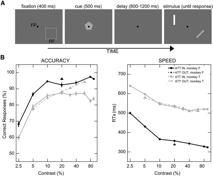
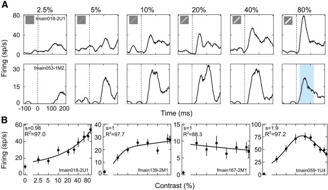
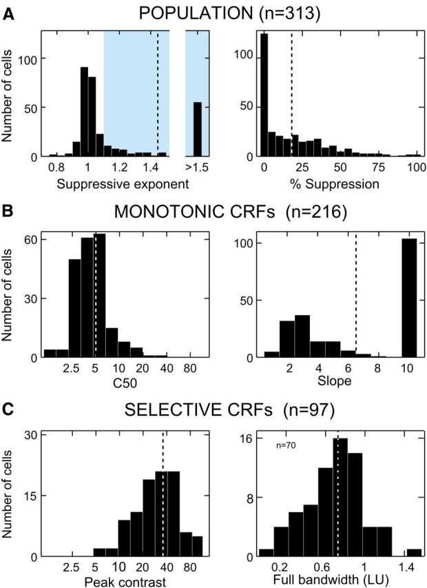
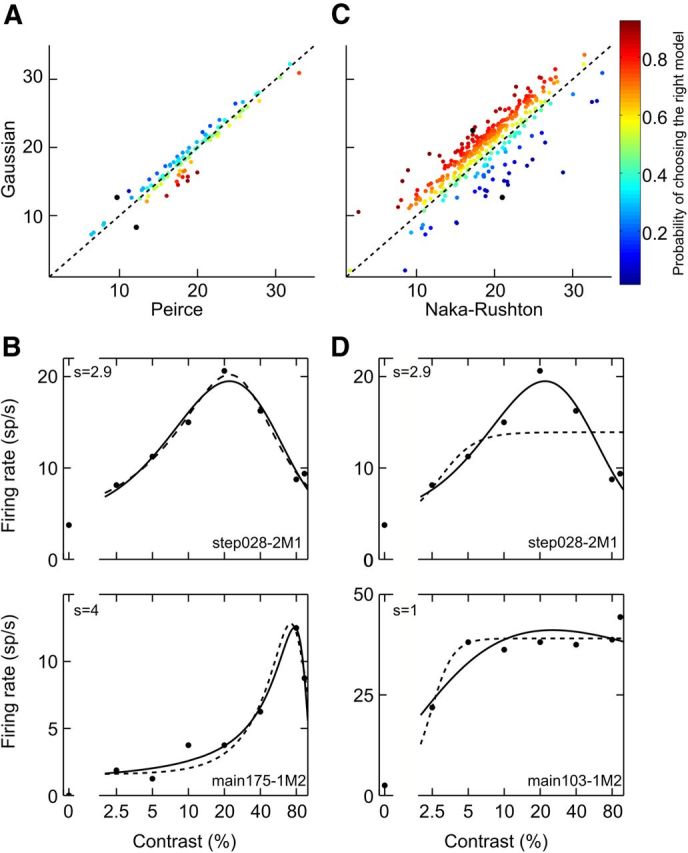
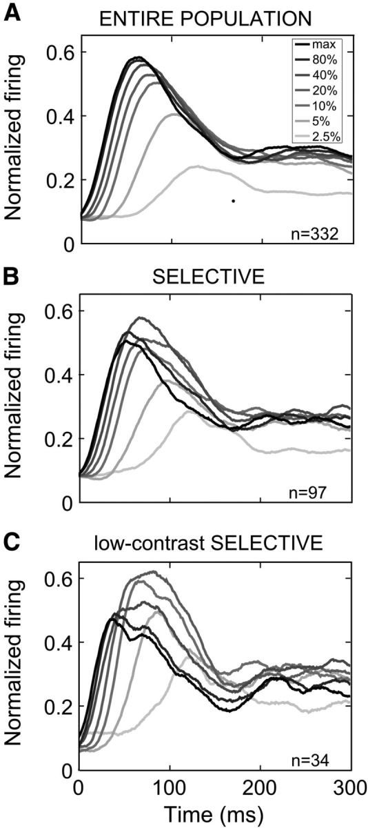
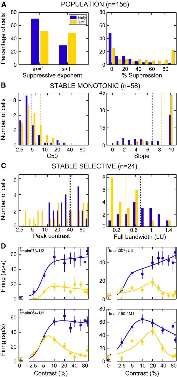
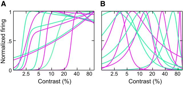
Visually responsive neurons typically exhibit a monotonic-saturating increase of firing with luminance contrast of the stimulus and are able to adapt to the current spatiotemporal context by shifting their selectivity, therefore being perfectly suited for optimal contrast encoding and discrimination. Here we report the first evidence of the existence of neurons showing selective tuning for contrast in area V4d of the behaving macaque (Macaca mulatta), i.e., narrow bandpass filter neurons with peak activity encompassing the whole range of visible contrasts and pronounced attenuation at contrasts higher than the peak. Crucially, we found that contrast tuning emerges after a considerable delay from stimulus onset, likely reflecting the contribution of inhibitory mechanisms. Selective tuning for luminance contrast might support multiple functions, including contrast identification and the attentive selection of low contrast stimuli.


Figures

Figure 1.
Figure 1.
Experimental paradigm and task performance. A, Behavioral task. The panels illustrate the temporal sequence of events within an example trial. The animal was trained to perform orientation discrimination on a bar stimulus located outside the RF of the neuron (top left quadrant); meanwhile, a bar was also displayed inside the RF at different contrast levels in two possible orientations. FP is the fixation point; RF indicates the classical RF; the pentagon represents the cue stimulus instructing the animal to allocate attention outside the RF; bars represent the stimuli to be discriminated; labels indicate the duration of each event in milliseconds. Note that the background is shown in gray for illustrative purposes (real luminance value, 2.49 cd/m2). B, Accuracy (percentage of correct responses) and mean reaction times (RTs) as a function of contrast (percentage Michelson contrast) are represented in the left and right, respectively. Solid and dashed lines, respectively, depict accuracy (or reaction times) for the orientation discrimination task performed inside and outside the RF of the neuron under study, separately for monkey F (in black) and monkey T (in gray). Only one data point is shown for monkey F in the attention-outside condition because the contrast was set to be constant (20%).
Figure 2.
Figure 2.
Response of V4 neurons to luminance contrast. A, PSTHs. PSTHs are plotted for six logarithmically spaced levels of contrast and aligned with stimulus onset for a monotonically increasing (top row) and a contrast-selective (bottom row) single-cell example. The light blue shaded area represents the 100 ms time window used for some of the analyses to calculate mean firing rate of the recorded cells. B, Monotonic increasing, monotonic saturating, non-modulated, and selective single-cell examples. Mean firing rate (spikes per seconds) is plotted as a function of percentage Michelson contrast. Each point represents the average of ≥12 stimulus presentations, along with its SEM (vertical lines). Solid lines depict the best fitted curve provided by the Peirce equation. s represents the value of the suppressive exponent given by the fitting procedures; note that this value is subsequently used to label cells as monotonic (s ≤ 1.1) or selective (s > 1.1; see Results).
Figure 3.
Figure 3.
Population and subpopulation properties of CRFs. A, Population. The panels show the distribution of the suppressive parameter (s), as given by each fitted Peirce function (median explained variance, 91.4%), and the percentage of suppression for each CRF, as derived from the Peirce function; the parameters are reported for all the well fitted neurons. The vertical dotted lines represent the average value of the depicted parameter. The light blue shaded area highlights the cells considered to be selective for contrast (s > 1.1). B, Parameter distribution for monotonic cells. The panels represent the distributions of C50, expressed in percentage Michelson contrast, and slope for the population of monotonic cells (s ≤ 1.1). Conventions as in A. C, Parameter distribution for selective cells. The panels represent the distributions of peak contrast and full bandwidth for the population of selective cells (s > 1.1), expressed in percentage Michelson contrast and log units (LU), respectively. Note that the bandwidth is reported for the selective cells showing at least 25% of inhibition (see Materials and Methods, Fitting procedures). Conventions as in A.
Figure 4.
Figure 4.
Consistency of classification of monotonic and selective CRFs. A, Peirce versus Gaussian function. The scatter plot depicts AIC values for the Gaussian function and the Peirce function fitted to the cells classified as selective for contrast according to the suppressive exponent (s) of the Peirce function (see Results, Heterogeneous CRFs in V4). Each data point represents a fitted neuron. The color of each point depicts the posterior probability to belong to one or the other of the two models; black dots represent the two neurons shown in B. Note that the lower the AIC value, the better is the fitting. B, Non-monotonic single-cell examples. Responses of two representative V4 neurons to bars of different contrast are shown. Mean firing rate (spikes per second) is calculated in a 100 ms time window starting at 40 ms after stimulus onset and is plotted as a function of percentage Michelson contrast. Each point represents the average of ≥12 stimulus presentations; the value of the suppressive exponent (s) calculated by fitting the Peirce function is reported for each cell. Lines depict the best fitted curve provided by the Peirce equation (dashed line) and the Gaussian equation (solid line). Note that the selected examples are two of the most extreme cases (more distant from the diagonal) in the scatter plot (A). C, Gaussian versus Naka–Rushton function. The scatter plot depicts AIC values for the Naka–Rushton function and the Gaussian function (convention as in A); black dots represent the two neurons shown in D. Note that low values of AIC indicate that the regression line properly fits the data. D, Monotonic saturating versus non-monotonic single-cell examples. Responses of two representative V4 neurons (reported in black in C) are shown (conventions as in B). Lines depict the best fitted curve provided by the Gaussian equation (solid line) and the Naka–Rushton equation (dashed line).
Figure 5.
Figure 5.
Population responses over time. Population PSTH for the preferred orientation is represented for each contrast level, aligned with stimulus onset (increasingly darker lines correspond to progressively higher contrasts). A, Average normalized PSTH for the entire population of recorded cells. B, Population PSTH for selective cells. C, Population PSTH for selective cells showing peak responses at low contrast levels (<20% Michelson contrast). Note that, for illustration purposes, 40 ms bin width has been used throughout. As indicated by the leftward shift of the PSTH, average latency decreased significantly as contrast increased, and this was true regardless of whether we considered the entire population of recorded neurons (F(6) = 126.82), the entire population of selective cells (F(6) = 40.6), or the subpopulation of selective cells having a peak for <20% contrast (F(6) = 9.21; p ≪ 0.01, 1-way ANOVA).
Figure 6.
Figure 6.
Changes in non-monotonicity over time. A, Average MI as a function of time, time locked to stimulus onset. MI, calculated in 20 ms time windows, shifted by 1 ms and averaged across the population, is plotted as a function of time for both the preferred (solid line) and unpreferred (dotted line) orientation. The population average OI (see Materials and Methods, Analysis of temporal dynamics) as a function of time is reported in red. Note that critical patterns for the two indices are coincident in time. B, Average MI over time, time locked to response onset (conventions as in A). The light blue shaded areas represent the two 50 ms time windows of maximal interest. C, Average MI over time for cells showing increasing or decreasing monotonicity. MI over time is reported separately for the subpopulation of cells with decreasing monotonicity (n = 209, solid line) and the subpopulation of cells with increasing monotonicity (n = 95, dotted line) as calculated from the comparison between the time windows of maximal interest. D–F, Single-cell examples. Average firing rate [spikes per second (sp/s)] of three representative neurons plotted as a function of contrast and time for 16 overlapping time epochs (50 ms width, 10 ms shift); surface color turns from blue to red for progressively higher discharge rate. Note that, with reference to C, single examples in D and E belong to the subpopulation of cells showing increasing non-monotonicity over time, whereas the example in F belongs to the subpopulation of cells with modestly decreasing non-monotonicity over time.
Figure 7.
Figure 7.
Changes in the shape of CRFs, early versus late windows. A, Entire population. In the left, the binomial distribution of the suppressive parameter (s) of well fitted neurons is shown separately for the early (in blue) and late (in yellow) time windows. The right represents the percentage of suppression of each well fitted CRF. The percentage of suppression increased significantly (p ≪ 0.01, two-tailed, paired t test) from an average value of 16 to 38%. B, Stably monotonic CRFs. The distributions of C50 (left) and slope (right) for the population of stably monotonic CRFs (s ≤ 1.1) is shown, separately for the early and late windows (conventions as in A). The blue and yellow vertical dotted lines represent the average C50 and slope for the early and late windows, respectively. C50 did not change significantly (p = 0.16, two-tailed, paired t test), whereas the slope increased significantly (p ≪ 0.01, two-tailed, paired t test). C, Stably selective cells. The distributions of peak contrast (left) and bandwidth (right) for the population of stably selective cells (s > 1.1) is shown, separately for the early and late windows (conventions as in A). Peak contrast did not change significantly (p = 0.72, two-tailed, paired t test), whereas the bandwidth was significantly reduced in the later window (p ≪ 0.01, two-tailed, paired t test). D, Single-cell examples. Responses of four representative V4 neurons to bars of different contrast are shown. Mean firing rate [spikes per second (sp/s)] is plotted as a function of percentage Michelson contrast for the early (in blue) and late (in yellow) windows, along with the best fitted curve provided by the Peirce function (solid lines).
Figure 8.
Figure 8.
Filtering properties in late epochs. Normalized responses (i.e., response − baseline, divided by the maximal response) of example neurons in the late time window (100–150 ms). A shows a set of 10 neurons showing a monotonic CRF, as described by the Peirce equation (s ≤ 1.1); note that most of the functions saturate or show some degree of supersaturation. B shows a set of 10 neurons characterized by a selective CRF, as described by the Peirce equation (s > 1.1); note that different neurons are selective for different contrast levels. For the sake of clarity, response functions are drawn in alternating colors along the contrast axis.
Figure 9.
Figure 9.
Contrast selectivity and eccentricity. The scatter plot depicts the RF center position within the visual field for all recorded neurons. Each cell was fitted by the Peirce function and classified as monotonic or selective according to the value of the suppressive exponent (see Results, Heterogeneous CRFs in V4; Fig. 3A). Gray and black dots correspond to neurons showing a monotonic or selective CRF, respectively. For the sake of visibility, neurons recorded at the same site are shifted by 0.05°. Note that contrast selectivity occurred at all levels of eccentricity, ranging from 2.53° to 9.11°. The number and the percentage of selective cells within each sector are reported.

Similar articles

Cited by

References

    1. Albrecht DG. Visual cortex neurons in monkey and cat: effect of contrast on the spatial and temporal phase transfer functions. Vis Neurosci. 1995;12:1191–1210. doi: 10.1017/S0952523800006817. - DOI - PubMed
    1. Albrecht DG, Hamilton DB. Striate cortex of monkey and cat: contrast response function. J Neurophysiol. 1982;48:217–237. - PubMed
    1. Albrecht DG, Geisler WS, Frazor RA, Crane AM. Visual cortex neurons of monkeys and cats: temporal dynamics of the contrast response function. J Neurophysiol. 2002;88:888–913. - PubMed
    1. Allman J, Miezin F, McGuinness E. Direction- and velocity-specific responses from beyond the classical receptive field in the middle temporal visual area (MT) Perception. 1985;14:105–126. doi: 10.1068/p140105. - DOI - PubMed
    1. Anderson JS, Lampl I, Gillespie DC, Ferster D. Membrane potential and conductance changes underlying length tuning of cells in cat primary visual cortex. J Neurosci. 2001;21:2104–2112. - PMC - PubMed

Publication types

LinkOut - more resources