Fibrinogen species as resolved by HPLC-SAXS data processing within the UltraScan Solution Modeler (US-SOMO) enhanced SAS module

Abstract

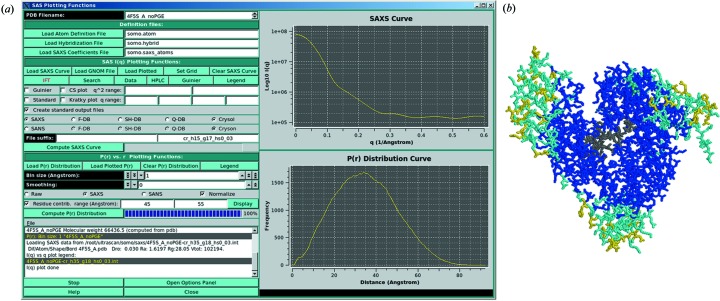
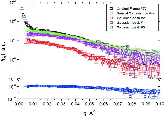
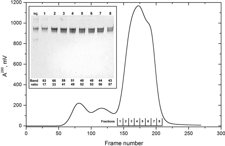
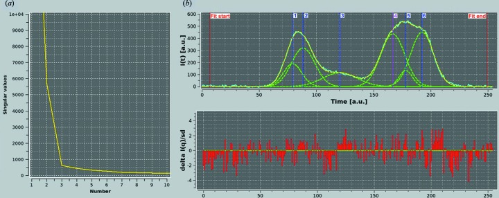
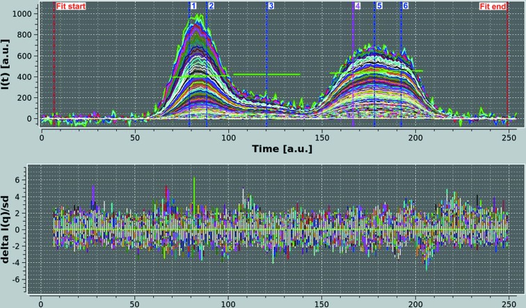
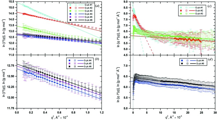
Fibrinogen is a large heterogeneous aggregation/degradation-prone protein playing a central role in blood coagulation and associated pathologies, whose structure is not completely resolved. When a high-molecular-weight fraction was analyzed by size-exclusion high-performance liquid chromatography/small-angle X-ray scattering (HPLC-SAXS), several composite peaks were apparent and because of the stickiness of fibrinogen the analysis was complicated by severe capillary fouling. Novel SAS analysis tools developed as a part of the UltraScan Solution Modeler (US-SOMO; http://somo.uthscsa.edu/), an open-source suite of utilities with advanced graphical user interfaces whose initial goal was the hydrodynamic modeling of biomacromolecules, were implemented and applied to this problem. They include the correction of baseline drift due to the accumulation of material on the SAXS capillary walls, and the Gaussian decomposition of non-baseline-resolved HPLC-SAXS elution peaks. It was thus possible to resolve at least two species co-eluting under the fibrinogen main monomer peak, probably resulting from in-column degradation, and two others under an oligomers peak. The overall and cross-sectional radii of gyration, molecular mass and mass/length ratio of all species were determined using the manual or semi-automated procedures available within the US-SOMO SAS module. Differences between monomeric species and linear and sideways oligomers were thus identified and rationalized. This new US-SOMO version additionally contains several computational and graphical tools, implementing functionalities such as the mapping of residues contributing to particular regions of P(r), and an advanced module for the comparison of primary I(q) versus q data with model curves computed from atomic level structures or bead models. It should be of great help in multi-resolution studies involving hydrodynamics, solution scattering and crystallographic/NMR data.

Keywords: HPLC-SAXS; bovine serum albumin; chromatography; fibrinogen; multi-resolution modeling; small-angle scattering.

Figure 1

(a) The renewed GUI of the US-SOMO SAS module main panel. In the graphic windows, the I(q) versus q and the P(r) versus r curves computed from the BSA crystal structure 4f5s (Bujacz, 2012 ▶) using Crysol and the US-SOMO internal SAXS method, respectively, are shown. (b) A snapshot of the RasMol-produced BSA structure with the residues contributing to the chosen P(r) versus r range, 45–55 Å, color coded from yellow to blue in order of decreasing importance.

Figure 2

Original frame #70 (top, black squares) of the SE-HPLC-SAXS BSA analysis (see Fig. S26), sum of the resulting I(q) versus q back generated from the Gaussians (green squares), and the contributions I(q) versus q of individual Gaussians for peak #2 (dimer; magenta squares) and peak #1 (trimer; red squares). Gaussian peak #3 (monomer; bottom, blue squares), does not contribute significantly to this frame.

Figure 3

(Main panel) UV chromatographic profile of an SE-HPLC-SAXS analysis of hpHMW-FG (20 µl at 17.3 mg ml⁻¹ in TBS were injected). (Inset) SDS/urea–PAGE analysis of the starting material (Inj.) and of the fractions collected on a duplicate run after disconnection from the SAXS setup (100 µl at ∼9 mg ml⁻¹ were injected). Fractions are indicated at the bottom of the main panel. Their concentration was determined, and equal amounts (∼1.9 µg for fractions 2–7, but only ∼1.2 µg for fractions 1 and 8) of not-reduced samples were loaded in the wells of a 10 × 8 cm 1.5 mm-thick 3.2% T–5% C polyacrylamide SDS/urea gel, electrophoresed, stained with Coomassie blue and subjected to densitometric analyses (see Cardinali et al., 2010 ▶). The fractional concentrations of the two main bands expressed in % are reported at the bottom of each lane.

Figure 4

(a) Plot of the first ten singular values versus value number derived from SVD analysis of the baseline-subtracted reconstructed I(q) versus q for the hpHMW-FG SE-HPLC-SAXS data set (q = 0.0030–0.170 Å⁻¹). (b) (Top graph) A single I(t) versus t chromatogram for q = 0.0058 Å⁻¹ (cyan), with the six fitting Gaussians (green curves, numbered 1–6 from left to right). The yellow curve is the sum of the Gaussians. (Bottom graph) The fit-associated reduced residuals.

Figure 5

(Top graph) Global Gaussians of the hpHMW-FG SE-HPLC-SAXS data [664 I(t) versus t data sets from q = 0.0030 Å⁻¹ to q = 0.170 Å⁻¹]. Six Gaussians were employed to fit the data, whose centers and widths are indicated by the vertical blue and magenta lines and by the green horizontal bars, respectively. (Bottom graph) The fit-associated reduced residuals.

Figure 6

(a) ln[I*(q)] versus q ² Guinier plots of the averaged and concentration/standard-normalized top peak frames for all the six Gaussian peaks derived from the decomposition of the hpHMW-FG SE-HPLC-SAXS data shown in Fig. 5 ▶. The data included in the linear regressions (straight lines) are indicated with filled symbols. All linear regressions were done with SD weighting with automatic rejection of outliers (set at ±2 SD) after definition of an appropriate q ² range, limited by the q _max R _g < 1.3 rule. (b) The Guinier plots for G-pks #4 (blue), #5 (magenta) and #6 (black) are shown on an expanded scale. (c), (d) Cross-section ln[qI*(q)] versus q ² Guinier plots for the same data as (a) and (b) (for the reason of clarity, G-pk #5 has been omitted, only one-half of the actual points are shown for all data sets, and the regression lines were prolonged at unphysical q ² < 0 values while the q ² = 0 axis is shown as a vertical gray line). Two linear regions were fitted, both limited by the q _max R _c < 1 rule, for G-pks #1 and #2 [(c), lower q ² range, dashed lines; higher q ²-range, solid lines], and one for all others [solid lines; G-pk #3, (c); G-pks #4 and #6, (d)].

References

1. Aster, R. C., Brochers, B. & Thurber, C. H. (2005). Parameter Estimation and Inverse Problems. Burlington, San Diego, London: Elsevier Academic Press.
1. Blombäck, B. (1996). Thromb. Res. 83, 1–75. - PubMed
1. Boccaccio, C. & Medico, E. (2006). Cell. Mol. Life Sci. 63, 1024–1027. - PMC - PubMed
1. Brookes, E., Demeler, B. & Rocco, M. (2010). Macromol. Biosci. 10, 746–753. - PubMed
1. Brookes, E., Demeler, B., Rosano, C. & Rocco, M. (2010). Eur. Biophys. J. 39, 423–435. - PMC - PubMed