Using networks to measure similarity between genes: association index selection

Abstract

Biological networks can be used to functionally annotate genes on the basis of interaction-profile similarities. Metrics known as association indices can be used to quantify interaction-profile similarity. We provide an overview of commonly used association indices, including the Jaccard index and the Pearson correlation coefficient, and compare their performance in different types of analyses of biological networks. We introduce the Guide for Association Index for Networks (GAIN), a web tool for calculating and comparing interaction-profile similarities and defining modules of genes with similar profiles.

Figure 1

Measuring interaction profile similarity between two nodes using association indices. (a) Bipartite graphs connect two types of nodes: X-type (purple) and Y-type (yellow). The interaction profile similarity between a pair of X-type nodes (A, B) is determined based on the number of shared Y-type nodes and the total number of Y nodes connected to A and B. (b) Association index comparison. For each pair of X-type nodes the Jaccard, Simpson, Geometric, Cosine, Hypergeometric indices and PCC were calculated based on their interactions with Y-type nodes. (c) CSI calculation between nodes A and B for a bipartite network involving six X-type nodes (purple) and seven Y-type nodes (yellow). For each pair of X-type nodes the PCC was calculated (blue, positive values; red, negative values). In the PCC association network all the edges connected to A or B are highlighted. CSI_AB represents the fraction of X-type nodes connected to both A and B with PCC < PCC_AB – 0.05. CSI was also calculated between A and C.

Figure 2

GAIN web tool for the calculation and clustering of association indices. (a) Screenshot of GAIN’s main window. (b) Visualization of a bipartite network as an interaction heatmap or (c) as a graph. (d) Clustered association index displayed as heatmap and (e) association network. (f) Density plot comparing the distribution of the association index values between a selected set of node pairs (blue) and all possible pairs of nodes (red).

Figure 3

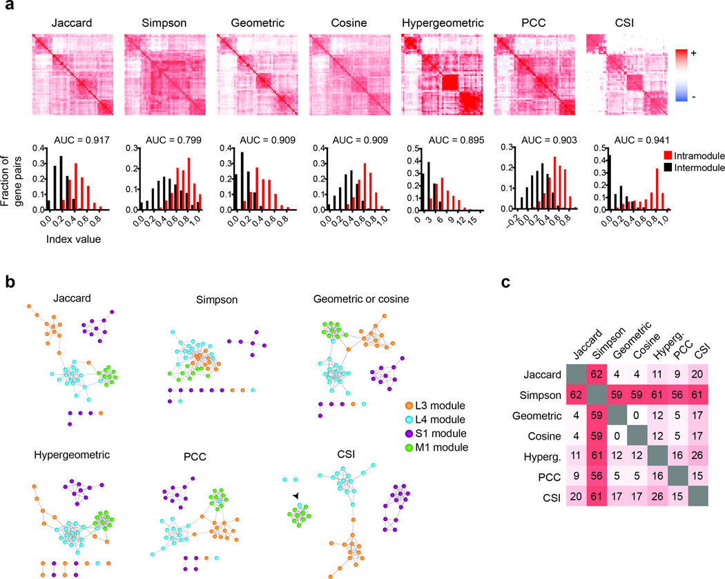
Using association indices to identify modules in a gene-to-phenotype network. (a) Clustered association index heatmaps for a C. elegans gene-to-phenotype network. The association index was calculated for each pair of genes according to shared phenotypic features and then clustered using hierarchical clustering. The distribution of index values for gene pairs that belong to the same module (intramodule, red) is plotted against the values of gene pairs that belong to different modules (intermodule, black). The area under the receiver operating characteristic curve (AUC) measures the separation between the two distributions. (b) Association networks were assembled by linking genes that have a top 10% phenotypic profile similarity value. A force-directed layout was generated by Cytoscape 2.8.1. The colors of the nodes represent a manual partitioning of the genes in modules. (c) Pair-wise comparison of the percentage of differences in the edges included in each of the association networks.

Figure 4

Comparing association indices in the C. elegans gene-to-phenotype network. (a, b) All pair-wise association index values for the genes according to shared phenotypic features for (a) the Simpson index and (b) CSI, plotted versus the values determined with the other indices. (c, d) The interaction profile similarity between (c) plc-1 and let-60 (belonging to different modules), (d) plc-1 and perm-3 (belonging to different modules) and between C47G2.3 and F57B10.1 (belonging to the same module) were determined for all the association indices. The ranking of interaction profile similarity across the entire network (in the top x% values) is indicated in the right. Yellow nodes indicate phenotypes. Phenotype hubs (connected to more than 40% of the genes) are indicated with a blue outline.

Figure 5

Predicting gene function. (a) A k-nearest neighbor (knn) algorithm was used to evaluate how well each index is able to assign genes to functional classes (F). To determine if an uncharacterized gene X can be assigned a particular function, a knn score was determined as the average of the top k association index (a.i.) values between X and genes with that function. The knn values were then calculated for genes with that function (blue and green) and for genes that do not have that function (black curves). To assign a function to gene X, the knn scores for genes that have that function and those that do not should be well separated. This separation was determined by calculating the AUC. The median AUC determined for all the functional classes was used as a measure of performance of the different association indices to predict gene function. The panel illustrates a case in which gene X can be assigned function 1 (F1, blue) but not function 2 (F2, green). (b) The median AUC calculated for the four functional classes in the C. elegans gene-to-phenotype network was determined for each value of k = 1 to 6 (number of nearest neighbors). (c) The median AUC calculated for the Biological Process GO slim terms in the yeast protein-DNA interaction network was determined for each value of k = 1 to 6 (number of nearest neighbors).

Figure 6

Application of association indices to network integration. (a) Using association indices, edges in one monopartite network can be compared to those in another, focusing either on a particular node (blue box) or on the entire network. (b) Comparing interaction profile similarity values in Network 1 between interacting and noninteracting nodes in Network 2. (c) The interaction profile similarity of the X-type nodes in Network 1 can be compared to the interaction profile similarity of the same nodes in Network 2. Edge width in the association network indicates is proportional to the association index value. (d) The association index values of C. elegans bHLH TFs was determined according to the tissues in which they are expressed, and was partitioned between proteins that physically interact (red) and those that do not (gray). Each box spans from the first to the third quartile, the horizontal line inside the box indicates the median value and the end of the whiskers indicate the minimum and maximum values. (e) Association index values were determined for pairs of promoters in the yeast protein-DNA interaction network. The values for pairs of highly coexpressed genes (red) and other gene pairs (gray) are plotted.

References

-
- Walhout AJM, et al. Protein interaction mapping in C. elegans using proteins involved in vulval development. Science. 2000;287:116–122. - PubMed
- Schwikowski B, Uetz P, Fields S. A network of protein-protein interactions in yeast. Nat. Genet. 2000;18:1257–1261. - PubMed
- Walhout AJM. Unraveling Transcription Regulatory Networks by Protein-DNA and Protein-Protein Interaction Mapping. Genome Res. 2006;16:1445–1454. - PubMed
Publication types
MeSH terms
Grants and funding
LinkOut - more resources
Full Text Sources
Other Literature Sources