Animal model of simulated microgravity: a comparative study of hindlimb unloading via tail versus pelvic suspension

Abstract

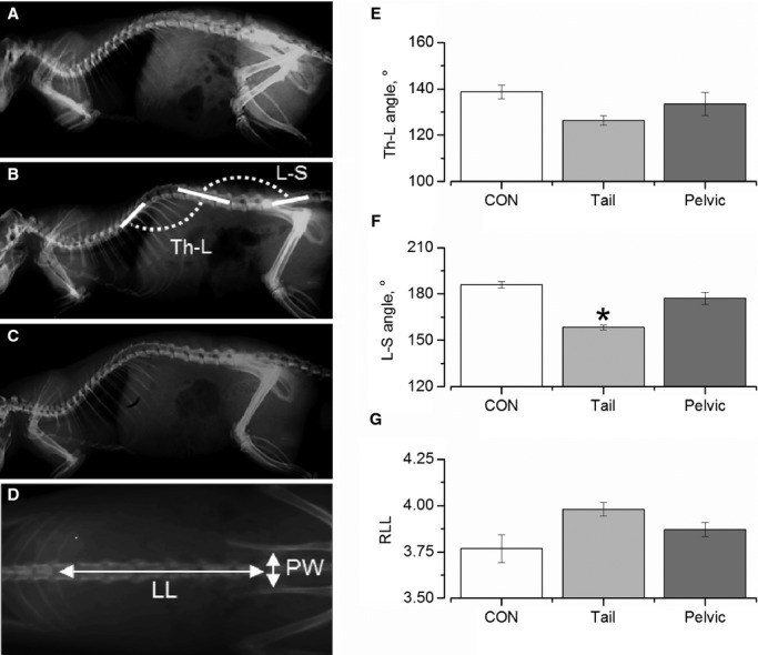
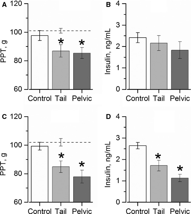
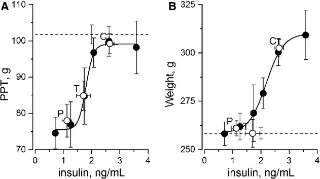
The aim of this study was to compare physiological effects of hindlimb suspension (HLS) in tail- and pelvic-HLS rat models to determine if severe stretch in the tail-HLS rats lumbosacral skeleton may contribute to the changes traditionally attributed to simulated microgravity and musculoskeletal disuse in the tail-HLS model. Adult male Sprague-Dawley rats divided into suspended and control-nonsuspended groups were subjected to two separate methods of suspension and maintained with regular food and water for 2 weeks. Body weights, food and water consumption, soleus muscle weight, tibial bone mineral density, random plasma insulin, and hindlimb pain on pressure threshold (PPT) were measured. X-ray analysis demonstrated severe lordosis in tail- but not pelvic-HLS animals. However, growth retardation, food consumption, and soleus muscle weight and tibial bone density (decreased relative to control) did not differ between two HLS models. Furthermore, HLS rats developed similar levels of insulinopenia and mechanical hyperalgesia (decreased PPT) in both tail- and pelvic-HLS groups. In the rat-to-rat comparisons, the growth retardation and the decreased PPT observed in HLS-rats was most associated with insulinopenia. In conclusion, these data suggest that HLS results in mild prediabetic state with some signs of pressure hyperalgesia, but lumbosacral skeleton stretch plays little role, if any, in these pathological changes.

Keywords: Hindlimb unloading; insulin; neuropathy; prediabetes; pressure hyperalgesia.

Figure 1

Pelvic hindlimb suspension technique and harness design. SS, suspension string; CA, central arc; LA, lower arm; BA, back arm.

Figure 2

Effects of 2 weeks of tail- and pelvic-HLS on rat axial skeleton. (A–D) Representative X-ray images of, respectively, control and tail- and pelvic-HLS rats and DEXA image of thorax-sacrum region of the control rat spine are shown. Such images were used to determine effects of HLS on rat spine curvature by measuring a thoracolumbar (Th-L) and lumbosacral (L-S) angles as illustrated in (B) and relative lumbar length (RLL) as illustrated in (D). The Th-L and L-S angles, measure of kyphosis and lordosis, were defined as respective angles between Th_8-11 and L_1-4, and L_1-4 and S_1-3 segments of spinal column. (E–G). Mean values of, respectively, Th-L and L-S angles and relative lumbar length (RLL) measured in control (white bars), and tail- (light gray) and pelvic- (dark gray) HLS rats. Number of studied animals is 3, 6, and 6 for control, tail-HLS and pelvic-HLS groups in (E) and (F), and 3, 6, and 16 for respective groups in (G). One way ANOVA with Tukey post hoc test reveals statistically significant effect on rat axial skeleton of tail-HLS only and only with respect to L-S angle (F; *P < 0.05 for tail-HLS vs. control comparisons by Tukey test).

Figure 3

Effects of 2 weeks of tail- and pelvic-HLS on the rat food (A) and water (B) consumption and weight gain (C). (A) Daily food consumption during a suspension period by control, tail-, and pelvic-HLS rats (n = 13, 6, and 12 animals per group, respectively. No between-group differences is detected by two-way repeated measures (RM) ANOVA at any of postsuspension day (F(2,84) = 0.44, P = 0.651). (B) Daily water consumption during a suspension period by control, tail-, and pelvic-HLS rats (n = 13, 6, and 12 animals per group, respectively). In the beginning of suspension period tail-HLS rats consume less food than either control or pelvic-HLS rats (asterisk; two-way RM ANOVA: F(2,84) = 3.50, P = 0.045; Bonferroni test: P < 0.01). (C) Body weight at baseline (day 0) and during suspension by control, tail-, and pelvic-HLS groups (n = 39, 18, and 21 animals per group, respectively). HLS results in net weight loss in tail-HLS (P < 0.05; days 3–7 vs. day 0; Tukey test) and in growth retardation in pelvic-HLS groups of animals. Later in experiment animal's weight gain by HLS rats resumes but control-HLS rats weight differences persist through entire 2 weeks of HLS period (between-group comparison by two-way RM ANOVA, followed by Bonferroni test; within-group comparisons by one-way RM ANOVA followed by Tukey test). All panels: closed, half-closed, and opened circles represent control, tail-HLS, and pelvic-HLS groups of rats, respectively.

Figure 4

Soleus muscle weight (A) and tibial bone mineral density (B) of control and hindlimb suspended rats. (A) Mean relative weight of soleus muscle of age-matched control, tail-, and pelvic-HLS rats (n = 12, 4, and 15 animals per group, respectively). Differences between control and tail- or pelvic-HLS groups are significant at P < 0.01 by one-way ANOVA with post hoc Tukey test. (B) Mean tibial bone mineral density (BMD) of age-matched control, tail-, and pelvic-HLS rats (n = 13, 12, and 8 animals per group, respectively). Differences between control and tail- or pelvic-HLS groups are significant at P < 0.01 by one-way ANOVA with post hoc Tukey test.

Figure 5

Pain on pressure threshold (A and C) and random plasma insulin concentration (B and D) measured in control and hindlimb suspended rats. (A) Pain on pressure thresholds (PPTs) measured at baseline (n = 90; horizontal dashed line) and after 2 weeks of the experiment in control and tail- and pelvic-HLS rats (n = 41, 26, and 23 animals per group, respectively). Both tail- and pelvic-HLS groups are statistically significantly different from the baseline PPT level (P < 0.01 by one-way ANOVA with post hoc Tukey test, asterisks). (B) Random plasma insulin concentration of control, tail-, and pelvic-HLS rats (n = 31, 15, and 17 animals per group, respectively). Between-group differences are not significant by one-way ANOVA with post hoc Tukey test. (C) Pain on pressure thresholds (filtered data, see text for the procedure) measured at baseline (n = 40; horizontal dashed line) and after 2 weeks of experiment in control and tail- and pelvic-HLS rats (n = 19, 8, and 13 animals per group, respectively). Both tail- and pelvic-HLS groups are statistically significantly different from both control and the experiment entry PPT levels (P < 0.01 by one-way ANOVA with post hoc Tukey test, asterisks). (D) Random plasma insulin concentration (filtered data, see text for the procedure) after 2 weeks of the experiment in control and tail- and pelvic-HLS rats (n = 19, 8, and 13 animals per group, respectively). Tail- and pelvic-HLS groups are statistically significantly different from control group (P < 0.01 by one-way ANOVA with post hoc Tukey test, asterisks). Filtering did not result in statistically significant changes of mean values of either PPT or insulin level in any of groups of animals (control, tail- or pelvic-HLS; P > 0.05, one-way ANOVA followed by Tukey test).

Figure 6

Insulin-PPT (A) and insulin-rat weight (B) relationships in control and HLS experiments. In both panels (the same as used in Fig. 5C and D) dataset of 40 animals was used. Filled circles represent mean PPT (A) and weight (B) values measured in groups of rats having random insulin levels within 0–1.0, 1.01–1.5, 1.51–2, 2.01–2.25, 2.26–3.00, and 3.01–4.0 ng/mL ranges (9, 4, 4, 9, 9, and 5 rats per respective range). Open circles represent mean characteristics of control and tail- and pelvic-HLS groups (19, 8, and 13 rats, “C,” “T,” and “P” text labels, respectively). Dashed lines represent mean baseline PPT (A) and weight (B) for all 40 rats studied. Solid curves are result of best fit of the Boltzmann equation (y = A2 + (A1 − A2)/(1 + exp([x − x0]/dx)) to the data shown by filled circles. The fit parameters are A1 = 75.0 ± 1.0 g, A2 = 99.1 ± 1.0 g, x0 = 1.80 ± 0.04 ng/mL, and dx = 0.13 ± 0.04 ng/mL (A: χ² = 1.739, adjusted R² = 0.986) and A1 = 259 ± 1 g, A2 = 310 ± 1 g, x0 = 2.19 ± 0.03 ng/mL, and dx = 0.31 ± 0.03 ng/mL (B: χ² = 1.346, adjusted R² = 0.997).

References

1. Allen MR, Hogan HA, Bloomfield SA. Differential bone and muscle recovery following hindlimb unloading in skeletally mature male rats. J. Musculoskelet. Neuronal Interact. 2006;6:217–225. - PubMed
1. Andersson G. Burden of musculoskeletal diseases in the United States: prevalence, societal and economic cost. Rosemont, IL: American Academy of Orthopaedic Surgeons; 2008.
1. Benedetti M, Merino R, Kusuda R, Ravanelli MI, Cadetti F, dos Santos P, et al. Plasma corticosterone levels in mouse models of pain. Eur. J. Pain. 2012;16:803–815. - PubMed
1. Bloomfield SA, Allen MR, Hogan HA, Delp MD. Site- and compartment-specific changes in bone with hindlimb unloading in mature adult rats. Bone. 2002;31:149–157. - PubMed
1. Carpenter RD, Lang TF, Bloomfield SA, Bloomberg JJ, Judex S, Keyak JH, et al. Effects of long-duration spaceflight, microgravity, and radiation on the neuromuscular, sensorimotor, and skeletal systems. J. Cosmol. 2010;12:3778–3780.
LinkOut - more resources