Functional analysis of ultra high information rates conveyed by rat vibrissal primary afferents

Abstract

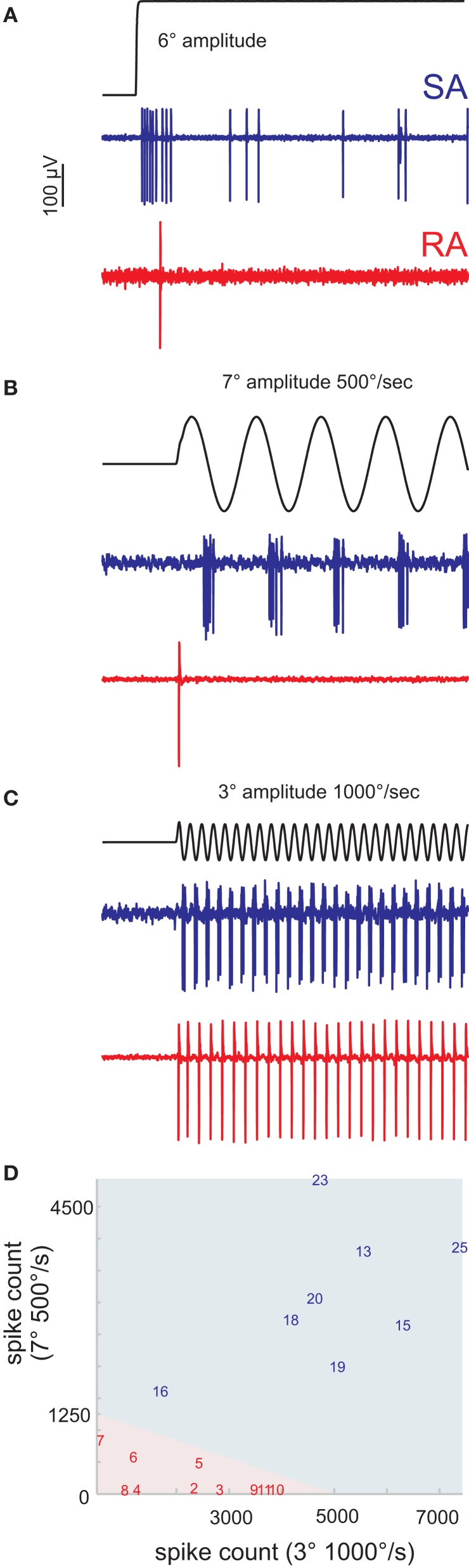
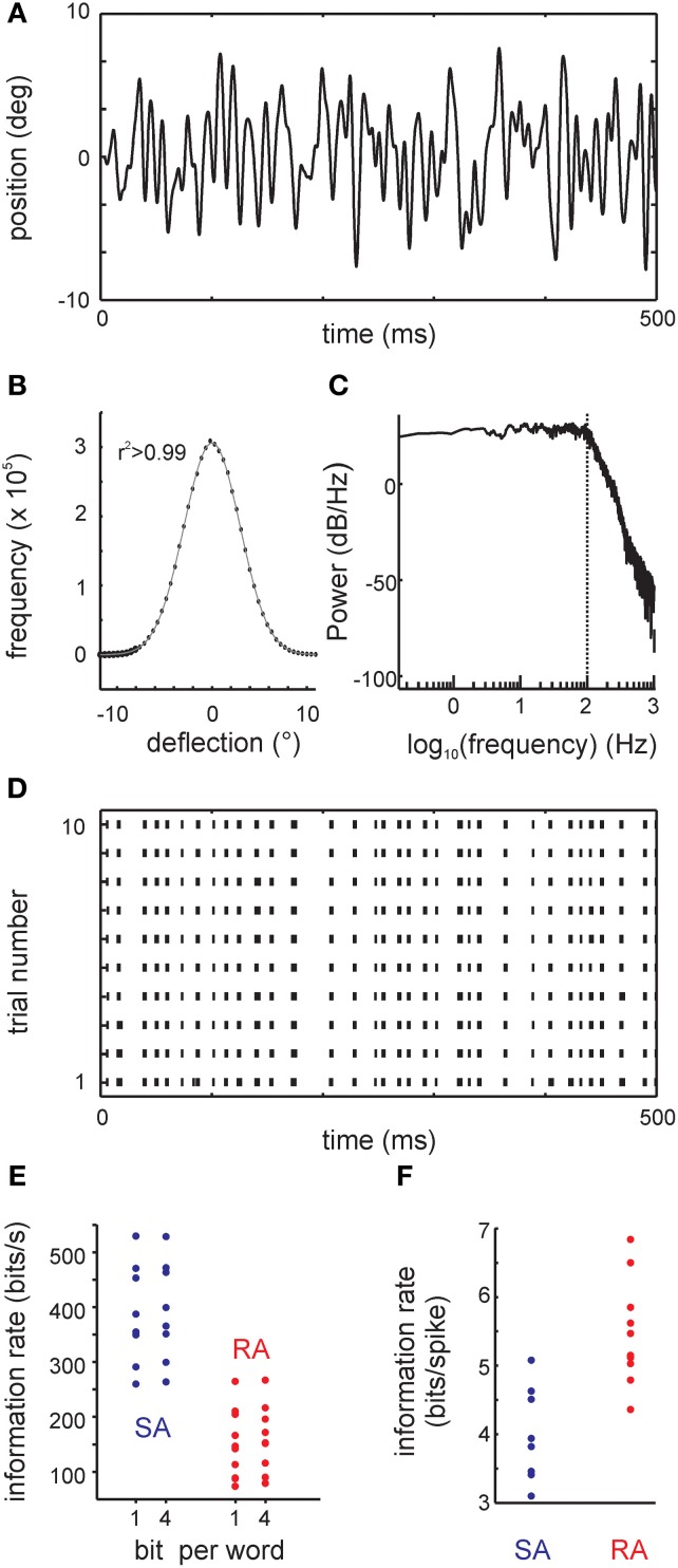
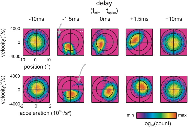
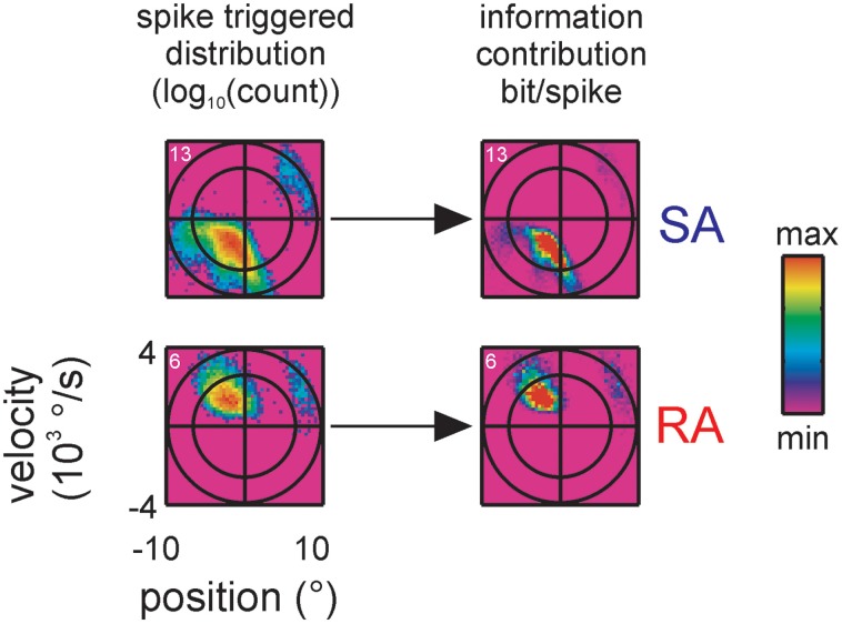
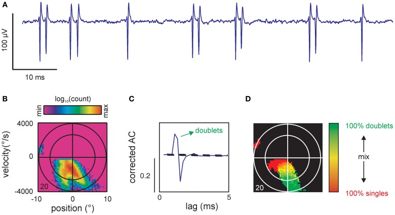
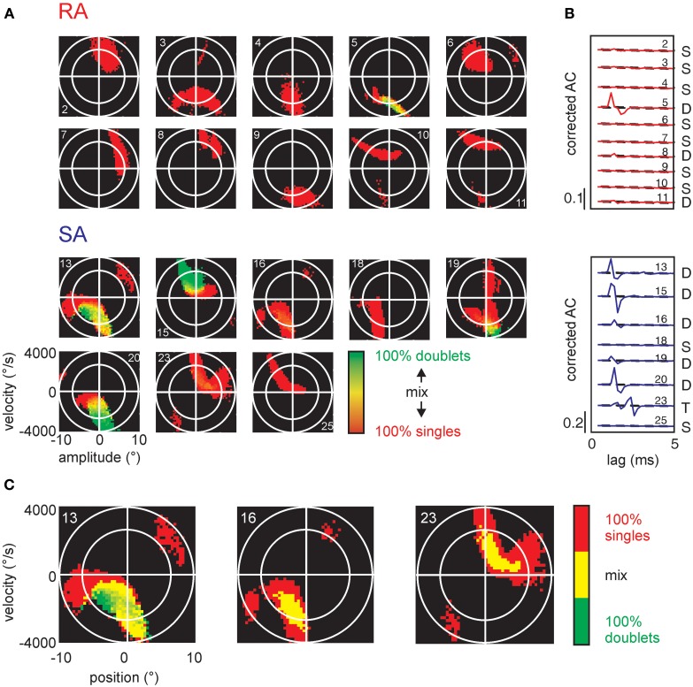
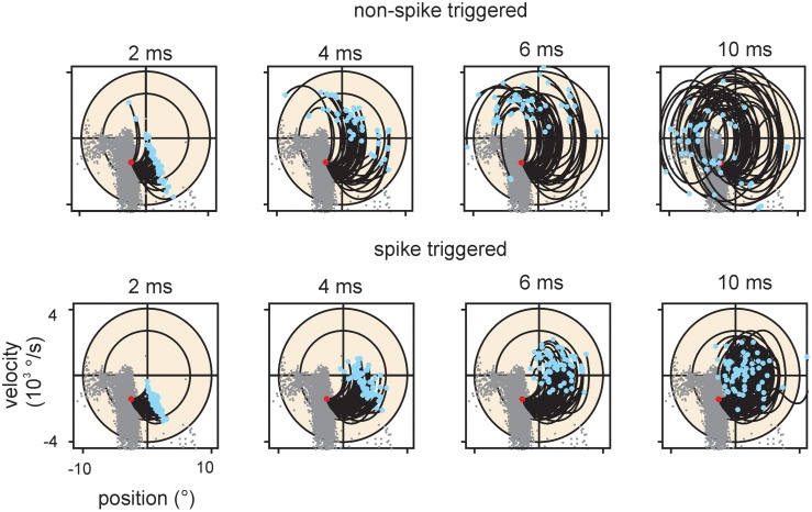
Sensory receptors determine the type and the quantity of information available for perception. Here, we quantified and characterized the information transferred by primary afferents in the rat whisker system using neural system identification. Quantification of "how much" information is conveyed by primary afferents, using the direct method (DM), a classical information theoretic tool, revealed that primary afferents transfer huge amounts of information (up to 529 bits/s). Information theoretic analysis of instantaneous spike-triggered kinematic stimulus features was used to gain functional insight on "what" is coded by primary afferents. Amongst the kinematic variables tested--position, velocity, and acceleration--primary afferent spikes encoded velocity best. The other two variables contributed to information transfer, but only if combined with velocity. We further revealed three additional characteristics that play a role in information transfer by primary afferents. Firstly, primary afferent spikes show preference for well separated multiple stimuli (i.e., well separated sets of combinations of the three instantaneous kinematic variables). Secondly, neurons are sensitive to short strips of the stimulus trajectory (up to 10 ms pre-spike time), and thirdly, they show spike patterns (precise doublet and triplet spiking). In order to deal with these complexities, we used a flexible probabilistic neuron model fitting mixtures of Gaussians to the spike triggered stimulus distributions, which quantitatively captured the contribution of the mentioned features and allowed us to achieve a full functional analysis of the total information rate indicated by the DM. We found that instantaneous position, velocity, and acceleration explained about 50% of the total information rate. Adding a 10 ms pre-spike interval of stimulus trajectory achieved 80-90%. The final 10-20% were found to be due to non-linear coding by spike bursts.

Keywords: information theory; primary afferents; rat; spike-triggered mixture model; tactile coding; vibrissae; whisker.

Figure 1

Classification of primary afferents. (A) Typical responses of rapidly (RA) and slowly adapting (SA) primary afferents to a ramp-and-hold stimulus in the preferred direction of the cell. (B,C) Discriminative responses of RA and SA units to sine waves of different amplitude and peak frequency. (B) Slow, high amplitude sine waves are not responded by RAs but by SAs. (C) Fast, low amplitude sine waves evoke responses in both cell classes. (D) A number of preliminary recordings were used to delineate the responses of RA and SA cells to the two sine wave stimuli (light red and blue background). The units reported in this study are labeled by a number. The numbering of cells and coloring (red/blue) according to cell class is consistent throughout all figures to allow the cross referencing of individual cells.

Figure 2

The filtered white noise stimulus and results obtained with a classical information theoretical analysis: the direct method (DM). (A) Example trace of the whisker's position. (B) The distribution of positions (circles) and the fit to a Gaussian (line). The coefficient of determination of the fit was r² > 0.99. (C) The stimulus power spectrum showing a flat density below 100 Hz (vertical dotted line). Above 100 Hz, there is a smooth roll-off. (D) Responses to the filtered white noise stimulus are very precise as demonstrated by the raster plot of one example primary afferent [response to the trace shown in (A)]. (E) Information rate (bit/s) calculated using DM for all cells in the sample. Information rate with bin width of 1 ms using 1 bit words (DM1.1) and 4 bit words (DM1.4) are shown. (F) Information rate converted into units of bits per spike (DM1.1).

Figure 3

Spike-triggered kinematic features. Two dimensional projections, taken from the 3D distributions of stimulus space spanned by position, velocity and acceleration, are shown. Top: position and velocity. Bottom: acceleration and velocity. The two ellipses (black lines, scales are chosen such that they appear as circles) indicate the total stimulus space (2 times and 3 times standard deviation of the 2D Gaussian). 2D histograms of the spike-triggered stimulus ensembles (color-coded) are plotted on top. Five delays between the occurrence of the spike and the stimulus feature are shown. At negative delays the spike follows the occurrence of the stimulus feature. Note the sharp and lobed sub-space (a separated preferred stimulus/lobe is marked by gray arrows) emerging when the stimulus is sampled 1.5 ms before the spike. (data of cell 20, cf. Figure 2D).

Figure 4

Encoded instantaneous stimulus features for our total sample of primary afferents. (A,B) original 3D stimulus space (as done in Figure 3). The spike-triggered stimulus ensembles found by maximizing the Kullback-Leibler Divergence (KLD) between stimulus distribution and spike-triggered stimulus ensemble are shown. Axis scaling and labeling is identical on all plots and is only shown once for clarity. The data pertaining to each cell are plotted onto a gray rectangle, the top plot depicts position vs. velocity, the bottom plot depicts acceleration vs. velocity. The cell numbers relating to Figure 2D are given in the top plots. (C) Average of one-dimensional projections onto the velocity axis showing different spike-triggered distributions of velocities in SA vs. RA cells distributions were sampled at each cell's optimal delay (cf. Figure 3).

Figure 5

Information contribution of extra lobes. Encoded stimulus features of two representative primary afferents containing multiple lobes, one SA (top, cell #13) and one RA (bottom, cell #6), are shown (conventions for axes and ellipsoid as in Figure 3). On the left, the spike triggered stimulus distributions are re-plotted from Figure 4 for comparison. On the right the information contribution of each stimulus bin is plotted (term within the sum operator in Equation 4). Information contribution of the extra lobe scales with the spike triggered distribution indicating that the sensitivity of the extra lobe does not grossly deviate from the one of the main lobe.

Figure 6

Spike patterns. (A) Voltage trace of single unit recording showing 2 single spikes and 5 doublets. (B) Spike-triggered stimulus ensemble of cell 20. (C) Corrected autocorrelogram (AC) showing a prominent peak far exceeding the prediction interval [PI, (5, 95%), broken lines]. The peak is followed by a trough departing below the PI likely indicating a refractory period after the second spike of the doublet. The ordinate scales correlation coefficient (r). Same cell as (B). (D) Coding of single spikes vs. doublets. Doublets were identified by searching the spike train for spike intervals corresponding to the interval as specified by the significant peak in the AC [cf. (C)]. To eliminate spurious spiking the map only contained color in bins that exceeded a total count of 5 events (spikes or doublets). Conventions for axes and ellipsoid in spike triggered ensembles as in Figure 3.

Figure 7

Stimulus encoding of single spikes and doublets for all cells in the sample. (A) Conventions as in Figure 6D, all cells in the sample. (B) Corrected autocorrelograms of all cells in the sample. Ordinate scales correlation coefficient (r). (C) The SA cells (numbers 13, 16, and 23) are re-plotted in a different color scheme to visualize the location of doublets and intermixed regions. Here, we only use three colors: pure single spike-triggered stimulus variables are colored red, pure doublet coding is shown in green, and stimulus-triggered by a mix of singles and doublets is colored yellow.

Figure 8

Encoding of stimulus trajectory. The graphs plot trajectories ending at a location in stimulus space within the main lobe of cell #18. Only the 2D projection spanning position and velocity is shown for clarity. Conventions for axes and ellipsoid in spike triggered ensembles as in previous figures. Trajectory start is marked by blue dots; trajectories end at the red dots. For reference the spike triggered instantaneous stimuli are depicted as gray dots in all graphs. Top row: Trajectories that did not evoke a spike. Bottom row: Trajectories that evoked a spike. All dots (gray, red, and blue) account for the optimal delay of the cell (cf. Figure 3). The duration of the trajectories is indicated above the graphs. Spike triggered trajectories (bottom) are more confined in the stimulus space as compared to the non-spike triggered ones (top), suggesting that the spikes carry trajectory information.

Figure 9

Generative encoding model based on mixtures of Gaussians (STM model). Model A. Non-linear features derived from the fits of spike-triggered and non-spike-triggered distributions by multiple Gaussians (boxes on the left) are linearly combined and the response passed through a sigmoid point non-linearity. The result determines the firing rate of the neuron. Model B. An extension of the model to incorporates spike-time dependencies. Log-densities of observing certain inter-spike intervals are plotted in the top right. The box on the lower right shows the log-density for observing intervals between a bin with no spike and a spike. The four log-likelihood terms are combined in a principled manner to give the firing rate of the neuron. For details of the model, see Theis et al. (2013).

Figure 10

Functional analysis of total information rate using the STM model. (A,B) Raster plots (left) and inter-spike interval distributions (ISI, right) as recorded (gray background), and generated by two probabilistic models (white background, cf. Figure 9). (A) Typical SA cell. Each row corresponds to one trial with the frozen white noise stimulus. Model A ignores the spike intervals. It reproduces the raster fairly well but introduces too many small intervals. Model B takes the spike intervals into account and clearly reproduces the cells' spike train better. Furthermore, it captures the refractory period and the doublet spiking of the cells better, as can be seen from the inter-spike-interval histograms (right). (B) Same as (A) but for a typical RA cell. (C,D). Comparison of information rate with DM1.1. Data from all cells; horizontal lines depict medians. (C) Information rate for instantaneous encoding of kinematic variables (p, position; v, velocity; a, acceleration). The information rate conveyed about combinations v, pv, and pva (that gave consistent and causally plausible delays of spikes following the stimulus and spikes) as normalized to the rate estimated by DM1.1 are shown. (D) Information rate relative to DM1.1 estimated using the STM model. Model A uses a 10 ms trajectory as input but ignores the spike history. The information rate is higher than in the instantaneous case but clearly lower than DM1.1. Accounting in addition for the last spike interval (Model B) results in information rates that are comparable with the ones obtained using DM1.1. The results plotted in lighter color were obtained from spike trains sampled during presentation of stimuli that were identical but roughly of half amplitude (3 standard deviations 5.1° instead of 10°, lines connect data points sampled from the same neurons).

Figure A1

Filter shapes estimated from spikes generated by one real and one artificial cell in response to a 100 Hz filtered white noise stimulus. (A,B) show filters obtained by fitting an STM to the responses of one SA cell. (C) The stimulus filter of a toy neuron (blue line) was estimated (black line) from the model's responses to the same stimulus as used in the experiments with real cells. Since we only used 10 principal component vectors to represent the filter, even a perfect estimate (yellow dashed line) would not have been able to recover the true filter. (D) Adding higher-frequency components allows us to represent the true filter but also increases the error in the estimated filter. (E) Amplitude spectra of the true filter (blue line) and the estimated filter (black solid line) of the toy neuron. The shaded region indicates a 90% confidence interval revealing high uncertainty in the high-frequency components of the estimated filter. The spectrum of the stimulus is shown as a gray line for reference (cf. Figure 2C).

Figure A2

Non-predictability of responses to simple stimuli from complex stimuli. (A,B) Responses to sine waves (on the ellipsoid track through the 2D kinematic space) and band-pass limited white noise of two example cells. (A) Primary afferent (SA, cell 16) that responded to the sine wave when entering both lobes as characterized by the broad-band stimulus. Such predictability was only seen in 2 cells (B) Another cell (RA, cell 11) did not respond when the sine wave traversed the second lobe (seen in 6 cells). (C,D) Same data but now plotted to reveal the velocity trajectory of broad-band and sine wave stimuli within the 10 ms interval preceding the spike. (C) Same cell as (A). The broad-band trajectories landing in the two lobes are depicted in light and medium blue color. The spike triggered sine wave trajectories are plotted in dark blue. (D) Same as (C), but for the cell shown in (B) (light and medium red: broad-band trajectories; dark red: sine wave trajectories). Here, in contrast to (C), sine waves landing in the lower lobe never elicit spikes.

References

1. Bialek W., Rieke F., De Ruyter Van Stefenick R. R., Warland D. (1991). Reading a neural code. Science 252, 1854–1857 10.1126/science.2063199 - DOI - PubMed
1. Bishop C. M. (2006). Pattern Recognition and Machine Learning. New York, NY: Springer
1. Borst A., Theunissen F. E. (1999). Information theory and neural coding. Nat. Neurosci. 2, 947–957 10.1038/14731 - DOI - PubMed
1. De Ruyter Van Steveninck R. R., Lewen G. D., Strong S. P., Koberle R., Bialek W. (1997). Reproducibility and variability in neural spike trains. Science 275, 1805–1808 10.1126/science.275.5307.1805 - DOI - PubMed
1. Deschenes M., Timofeeva E., Lavallee P. (2003). The relay of high-frequency sensory signals in the Whisker-to-barreloid pathway. J. Neurosci. 23, 6778–6787 - PMC - PubMed
Publication types
LinkOut - more resources