

Searching for collective behavior in a large network of sensory neurons
- PMID: 24391485
- PMCID: PMC3879139
- DOI: 10.1371/journal.pcbi.1003408
Searching for collective behavior in a large network of sensory neurons
Abstract
Maximum entropy models are the least structured probability distributions that exactly reproduce a chosen set of statistics measured in an interacting network. Here we use this principle to construct probabilistic models which describe the correlated spiking activity of populations of up to 120 neurons in the salamander retina as it responds to natural movies. Already in groups as small as 10 neurons, interactions between spikes can no longer be regarded as small perturbations in an otherwise independent system; for 40 or more neurons pairwise interactions need to be supplemented by a global interaction that controls the distribution of synchrony in the population. Here we show that such "K-pairwise" models--being systematic extensions of the previously used pairwise Ising models--provide an excellent account of the data. We explore the properties of the neural vocabulary by: 1) estimating its entropy, which constrains the population's capacity to represent visual information; 2) classifying activity patterns into a small set of metastable collective modes; 3) showing that the neural codeword ensembles are extremely inhomogenous; 4) demonstrating that the state of individual neurons is highly predictable from the rest of the population, allowing the capacity for error correction.
Conflict of interest statement
The authors have declared that no competing interests exist.
Figures
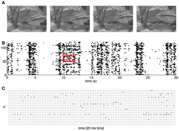
 represents a silence (absence of spike) of neuron i, and
  represents a spike.
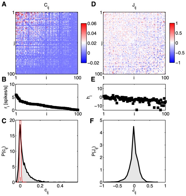
 , (B) firing rates (equivalent to
  ), and (C) the distribution of correlation coefficients
  . The red distribution is the distribution of differences between two halves of the experiment, and the small red error bar marks the standard deviation of correlation coefficients in fully shuffled data (1.8×10⁻³). At right, the parameters of a pairwise maximum entropy model [
 from Eq (19)] that reproduces these data: (D) coupling constants
  , (E) fields
  , and (F) the distribution of couplings in this group of neurons.
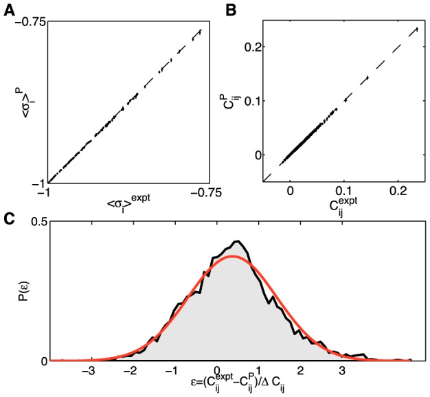
 covariance matrix elements, normalized by the estimated error bar in the data; red overlay is a Gaussian with zero mean and unit variance. The distribution has nearly Gaussian shape with a width of ≈1.1, showing that the learning algorithm reconstructs the covariance statistics to within measurement precision.
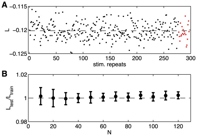
 ) under the pairwise model of Eq (19), computed on the training repeats (black dots) and on the testing repeats (red dots), for the same group of N = 100 neurons shown in Figure 1 and 2. Here the repeats have been reordered so that the training repeats precede testing repeats; in fact, the choice of test repeats is random. (B) The ratio of the log-likelihoods on test vs training data, shown as a function of the network size N. Error bars are the standard deviation across 30 subgroups at each value of N.
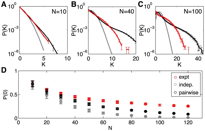
 for subnetworks of size
  ; error bars are s.d. across random halves of the duration of the experiment. For N = 10 we already see large deviations from an independent model, but these are captured by the pairwise model. At N = 40 (B), the pairwise models miss the tail of the distribution, where
  . At N = 100 (C), the deviations between the pairwise model and the data are more substantial. (D) The probability of silence in the network, as a function of population size; error bars are s.d. across 30 subgroups of a given size N. Throughout, red shows the data, grey the independent model, and black the pairwise model.
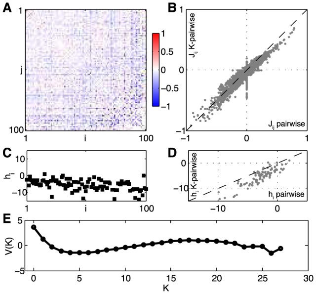
 , and the comparison with the interactions of the pairwise model, (B). (C) Single-neuron fields,
  , and the comparison with the fields of the pairwise model, (D). (E) The global potential, V(K), where K is the number of synchronous spikes. See Methods: Parametrization of the K-pairwise model for details.
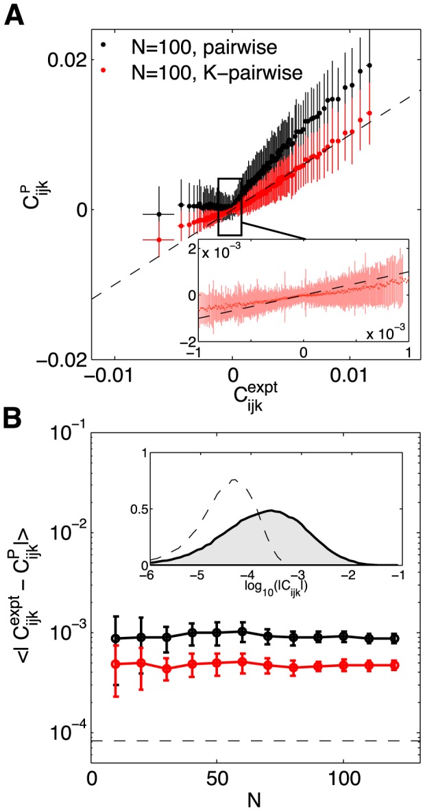
 (x-axis) vs predicted by the model (y-axis), shown for an example 100 neuron subnetwork. The ∼1.6×10⁵ triplets are binned into 1000 equally populated bins; error bars in x are s.d. across the bin. The corresponding values for the predictions are grouped together, yielding the mean and the s.d. of the prediction (y-axis). Inset shows a zoom-in of the central region, for the K-pairwise model. (B) Error in predicted three-point correlation functions as a function of subnetwork size N. Shown are mean absolute deviations of the model prediction from the data, for pairwise (black) and K-pairwise (red) models; error bars are s.d. across 30 subnetworks at each N, and the dashed line shows the mean absolute difference between two halves of the experiment. Inset shows the distribution of three–point correlations (grey filled region) and the distribution of differences between two halves of the experiment (dashed line); note the logarithmic scale.
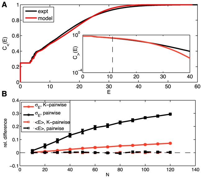
 from Eq (22), for the K-pairwise models (red) and the data (black), in a population of 120 neurons. Inset shows the high energy tails of the distribution,
  from Eq (24); dashed line denotes the energy that corresponds to the probability of seeing the pattern once in an experiment. See Figure S5 for an analogous plot for the pairwise model. (B) Relative difference in the first two moments (mean,
  , dashed; standard deviation,
  , solid) of the distribution of energies evaluated over real data and a sample from the corresponding model (black = pairwise; red = K-pairwise). Error bars are s.d. over 30 subnetworks at a given size N.
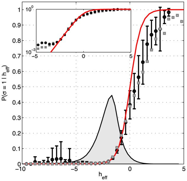
 neurons, the K-pairwise model predicts the probability of firing of the N-th neuron by Eqs (25,26); the effective field
  is fully determined by the parameters of the maximum entropy model and the state of the network. For each activity pattern in recorded data we computed the effective field, and binned these values (shown on x-axis). For every bin we estimated from data the probability that the N-th neuron spiked (black circles; error bars are s.d. across 120 cells). This is compared with a parameter-free prediction (red line) from Eq (26). For comparison, gray squares show the analogous analysis for the pairwise model (error bars omitted for clarity, comparable to K-pairwise models). Inset: same curves shown on the logarithmic plot emphasizing the low range of effective fields. The gray shaded region shows the distribution of the values of
  over all 120 neurons and all patterns in the data.
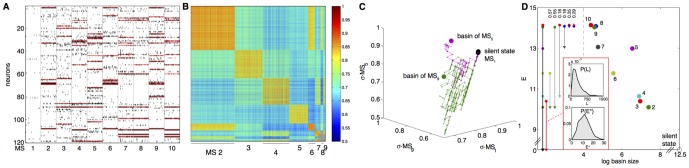
 , between all pairs of identified patterns belonging to basins 2,…,10 (MS 1 left out due to its large size). Patterns within the same basin are much more similar between themselves than to patterns belonging to other basins. (C) The structure of the energy landscape explored with Monte Carlo. Starting in the all-silent state, single spin-flip steps are taken until the configuration crosses the energy barrier into another basin. Here, two such paths are depicted (green, ultimately landing in the basin of MS 9; purple, landing in basin of MS 5) as projections into 3D space of scalar products (overlaps) with the MS 1, 5, and 9. (D) The detailed structure of the energy landscape. 10 MS patterns from (A) are shown in the energy (y-axis) vs log basin size (x-axis) diagram (silent state at lower right corner). At left, transitions frequently observed in MC simulations starting in each of the 10 MS states, as in (C). The most frequent transitions are decays to the silent state. Other frequent transitions (and their probabilities) shown using vertical arrows between respective states. Typical transition statistics (for MS 3 decaying into the silent state) shown in the inset: the distribution of spin-flip attempts needed, P(L), and the distribution of energy barriers,
  , over 1000 observed transitions.
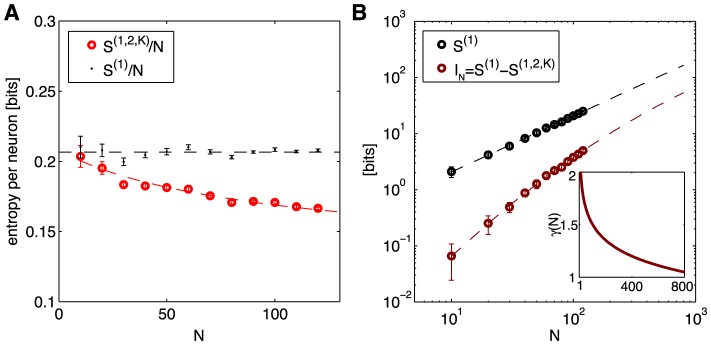
 , in black, and the entropy of the K-pairwise models per neuron,
  , in red, as a function of N. Dashed lines are fits from (B). (B) Independent entropy scales linearly with N (black dashed line). Multi-information
  of the K-pairwise models is shown in dark red. Dashed red line is a best quadratic fit for dependence of
  on
on  ; this can be rewritten as
  , where γ(N) (shown in inset) is the effective scaling of multi-information with system size N. In both panels, error bars are s.d. over 30 subnetworks at each size N.
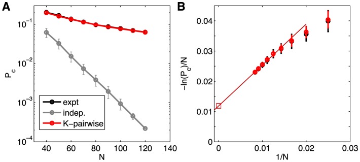
 to large N.
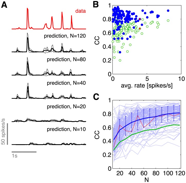
References
-
- Amit DJ (1989) Modeling Brain Function: The World of Attractor Neural Networks. Cambridge: Cambridge University Press.
-
- Hertz J, Krogh A & Palmer RG (1991) Introduction to the Theory of Neural Computation. Redwood City: Addison Wesley.
Publication types
MeSH terms
Grants and funding
LinkOut - more resources
Full Text Sources
Other Literature Sources
