Sparsity-regularized HMAX for visual recognition

Abstract

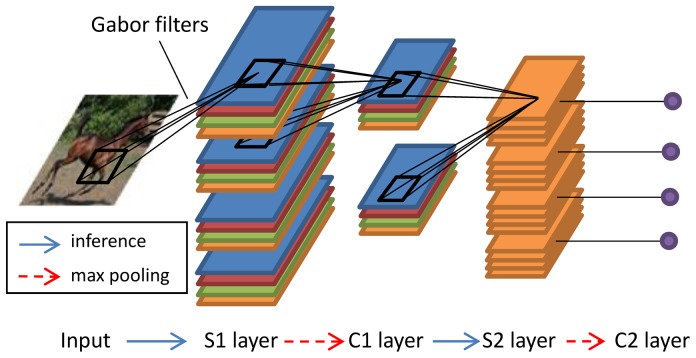
About ten years ago, HMAX was proposed as a simple and biologically feasible model for object recognition, based on how the visual cortex processes information. However, the model does not encompass sparse firing, which is a hallmark of neurons at all stages of the visual pathway. The current paper presents an improved model, called sparse HMAX, which integrates sparse firing. This model is able to learn higher-level features of objects on unlabeled training images. Unlike most other deep learning models that explicitly address global structure of images in every layer, sparse HMAX addresses local to global structure gradually along the hierarchy by applying patch-based learning to the output of the previous layer. As a consequence, the learning method can be standard sparse coding (SSC) or independent component analysis (ICA), two techniques deeply rooted in neuroscience. What makes SSC and ICA applicable at higher levels is the introduction of linear higher-order statistical regularities by max pooling. After training, high-level units display sparse, invariant selectivity for particular individuals or for image categories like those observed in human inferior temporal cortex (ITC) and medial temporal lobe (MTL). Finally, on an image classification benchmark, sparse HMAX outperforms the original HMAX by a large margin, suggesting its great potential for computer vision.

Figure 1. Illustration of HMAX.

Inference is realized by template matching. Different colors in S1 and C1 layers correspond to four different orientations of Gabor filters.

Figure 2. Illustration of the first two layers of HMAX.

The subscripts denote filter labels and the superscripts denote positions. Max pooling is only applied over positions.

Figure 3. Statistics of correlation coefficients.

First column: correlations between responses of different filters at the same location. Second column: correlations between responses of the same filter at different locations. Third column: correlations between responses of different filters at different locations. The distance between locations is pixels on the original image space. First row: results on the S1 layer in Figure 2. Second to fourth rows: results on the C1 layer in Figure 2 with max pooling, average pooling and square pooling, respectively, where the pooling ratio . Fifth row: mean of the absolute values of correlation coefficients with respect to the pooling ratio , where the open circles, asterisks and squares denote max pooling, average pooling and square pooling, respectively.

Figure 4. Illustration of sparse HMAX with six layers.

Figure 5. Visualization of S1 bases (left), S2 bases (middle) and S3 bases (right) learned on the Kyoto dataset.

Figure 6. Visualization of S2 bases (bottom) and S3 bases (top) learned on the Caltech-101 dataset.

From left to right, the columns display results on images from four categories: faces-easy, car-side, elephant and ibis, respectively.

Figure 7. Visualization of S3 bases learned on images from mixed categories of the Caltech-101 dataset: faces-easy, car-side, elephant and ibis.

Figure 8. Representation for different individuals.

First row: most selective units to ten individuals. Second row: ROC of these units for identifying the corresponding individuals. Horizontal axis: false positive rate. Vertical axis: true positive rate. Third and fourth rows: images that induced highest responses to the first and second units shown in the first row, respectively. The number above each image is the response value of the corresponding unit.

Figure 9. Representation for general categories.

First row: most selective units to the four categories. Second row: ROC of these units for identifying the corresponding categories. Horizontal axis: false positive rate. Vertical axis: true positive rate. Third to sixth rows: images that induced highest responses to the four units shown in the first row, respectively. The number above each image is the response value of the corresponding unit.

Figure 10. Training and testing on a mixture of LFW data and ImageNet data.

(a) Bases of six face-sensitive units with their test accuracies indicated above. (b) The histogram of the activation values of the best unit (the rightmost in (a)) for 5,000 positive samples (blue) and 5,000 negative samples (red). (c) 36 images that elicited greatest activations for the best unit.

Figure 11. A sample sequence of horizontal occlusions (top) and vertical occlusions (bottom).

All of the occlusion portions shown here correspond to the activation values above the threshold of the second best unit (see the last row of Figure 12).

Figure 12. Average activation value of the second best unit on distorted images.

Dashed line indicates the threshold.

Figure 13. Classification accuracy of the L2-regularized HMAX with respect to different values of the regularization parameter

on the Caltech-101 dataset. The curve shows the average results over ten random splits of train/test samples and the error bars show the standard deviations. The x-axis is in the log scale.

References

-
- Pasupathy A, Connor CE (2002) Population coding of shape in area V4. Nature Neuroscience 5: 1332–1338. - PubMed
- Fukushima K (1980) Neocognitron: A self-organizing neural network model for a mechanism of pattern recognition unaffected by shift in position. Biological Cybernetics 36: 193–202. - PubMed
- Riesenhuber M, Poggio T (1999) Hierarchical models of object recognition in cortex. Nature Neuroscience 2: 1019–1025. - PubMed
Publication types
MeSH terms
LinkOut - more resources
Full Text Sources
Other Literature Sources
Research Materials
Miscellaneous