Mechanisms for similarity matching in disparity measurement

Abstract

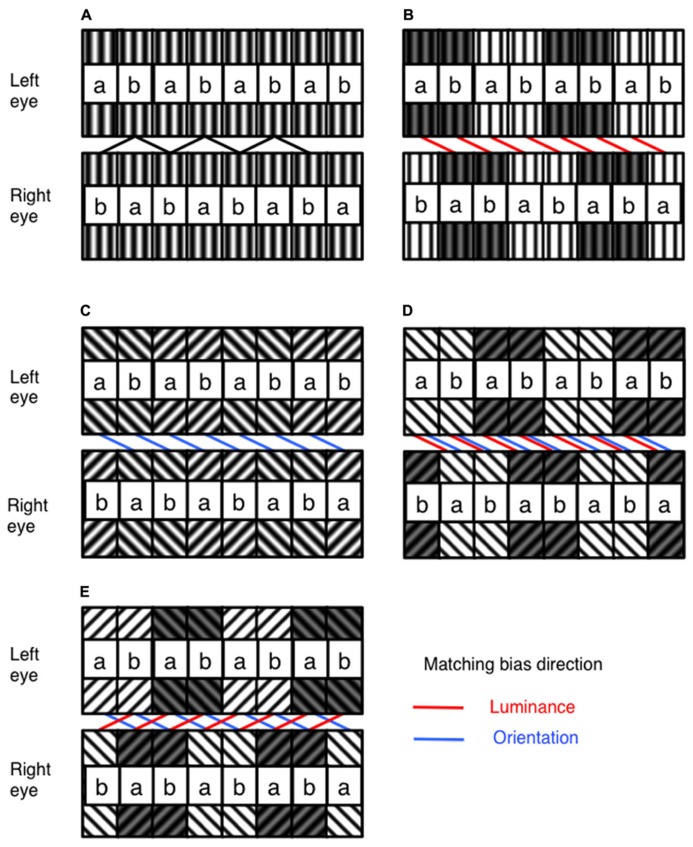
Early neural mechanisms for the measurement of binocular disparity appear to operate in a manner consistent with cross-correlation-like processes. Consequently, cross-correlation, or cross-correlation-like procedures have been used in a range of models of disparity measurement. Using such procedures as the basis for disparity measurement creates a preference for correspondence solutions that maximize the similarity between local left and right eye image regions. Here, we examine how observers' perception of depth in an ambiguous stereogram is affected by manipulations of luminance and orientation-based image similarity. Results show a strong effect of coarse-scale luminance similarity manipulations, but a relatively weak effect of finer-scale manipulations of orientation similarity. This is in contrast to the measurements of depth obtained from a standard cross-correlation model. This model shows strong effects of orientation similarity manipulations and weaker effects of luminance similarity. In order to account for these discrepancies, the standard cross-correlation approach may be modified to include an initial spatial frequency filtering stage. The performance of this adjusted model most closely matches human psychophysical data when spatial frequency filtering favors coarser scales. This is consistent with the operation of disparity measurement processes where spatial frequency and disparity tuning are correlated, or where disparity measurement operates in a coarse-to-fine manner.

Keywords: binocular energy model; binocular vision; correspondence problem; cross-correlation; disparity measurement; similarity.

FIGURE 1

Illustration of the general structure of the stimulus, and the manipulation of luminance and orientation ambiguity. (A) The stimulus is built from tiles of filtered random dot textures, a and b. In one eye, these are arranged in a repeating ab sequence. In the other eye, they are arranged in a repeating ba sequence. With no difference in luminance or orientation, these stimuli can equally be matched with a crossed or uncrossed disparity (B) With the addition of a difference in luminance between pairs of ab units in each stimulus, matching can be biased toward a particular disparity. (C) Similarity in orientation between corresponding ab pairings can also be used to bias disparity matching. Luminance and orientation similarity can be introduced so as to bias in (D) the same or (E) competing directions. The direction of matching based on similarity in luminance and orientation are indicated by the red and blue lines on the figures, respectively. Spatial frequencies for the experimental stimuli were identical across all orientation and luminance similarities, and are shown in this figure for illustrative purposes only. The labeling of ab pairings indicated in this figure were not present in actual experimental stimuli.

FIGURE 2

Examples of the experimental stimuli. Since stimuli are periodic, either crossed or parallel fusion of left and right columns will demonstrate the effects of manipulating similarity-based matching. White vertical lines indicate the plane of fixation. Examples of experimental stimuli are shown for each case from Figure 1. (A) An example stimulus containing no luminance or orientation bias. (B) Matching is biased through manipulation of luminance similarity only. (C) Matching is biased through manipulation of orientation similarity only. (D) Manipulations of orientation and luminance similarity are applied in the same direction. (E) Manipulations of orientation and luminance similarity are applied in opposite directions.

FIGURE 3

The cross-correlation model. (A) Illustration of the correlation window size relative to the experimental stimulus. Using correlation windows greater in size than the range of similarity manipulations ensures that normalization of mean luminance does not degrade model performance. Offset in window positions shows a disparity shift consistent with the periodic structure of the stimulus. (B) Output of the standard cross-correlation model. Results show the correlation as a function of disparity. The black line shows the results with no luminance bias. This shows peaks in the correlation function of equal magnitude for crossed and uncrossed disparities. Outputs are also shown for a luminance bias of 0.25 (red line) and 0.5 (blue line). As the luminance bias increases, the correlation increases for one sign of disparity, and decreases for the other. Note that, although the output of the correlation model is shown here at a range of disparities, the decision stage of the model only considers disparities consistent with the periodic structure of the stimulus.

FIGURE 4

Psychophysical results for author PH (lefthand column), author RG (central column), and the naïve observer (righthand column). (A–C) show the proportion of “far” results as a function of the luminance bias. Separate lines indicate the results for each level of orientation similarity, as indicated by the legend. A clear effect of luminance similarity is evident for all levels of orientation similarity. (D–F) show the results plotted as a function of orientation bias. When matching is not biased by luminance similarity (the cyan curve) a clear effect of orientation is evident for all three observers. With a large luminance matching bias, orientation has little or no effect on disparity matching. (G–I) plot the psychophysical data as a heat-map to illustrate the full two-dimensional psychometric function. The color of the pixels indicates the proportion of “far” responses.

FIGURE 5

Results of the cross-correlation model. Top row: The mean of the psychophysical results plotted in Figure 4, across the three observers. Results are plotted (A) as a function of luminance bias (B) as a function of orientation bias and (C) as a two-dimensional heat-map, where color shows the proportion of “far” responses. Second row (D–F): The results of the standard cross-correlation model. Unlike the psychophysical results, the model shows a strong effect of orientation, and an effect of luminance only when there is no orientation bias. Third row (G–I): The results of a cross-correlation model after filtering at a low spatial frequency (0.47 cpd). The model now shows a strong effect of luminance bias, and a weaker effect of orientation bias. Fourth row (J–L): The results of a cross-correlation model after filtering at a high spatial frequency (3.79 cpd). This model shows a strong effect of orientation and a weaker effect of luminance. Fifth row (M–O): The correlation model with filtering at 1.4 cpd shows the closest fit to the psychophysical data.

FIGURE 6

Differences between the psychophysical data and the model results for (A) the standard correlation model and (B) the best-fitting correlation model. Color indicates the difference in proportion of “far” responses between the models and the averaged human psychophysical data. These differences are summarized in (C), which shows the sum-of-squared differences between the psychophysical and model data as a function of the spatial frequency of filtering. The horizontal line shows the result for the standard cross-correlation model with no filtering. (D) An example of a luminance biased stimulus in original (top row) and filtered (bottom row) states. The filter applied has a spatial frequency of 1.4 cpd, which corresponds to that used in the best-fitting model.

References

1. Allenmark F, Read J. C. A. (2010). Detectability of sine- versus square-wave disparity gratings: a challenge for current models of depth perception. J. Vis. 10:17 10.1167/10.8.17 - DOI - PubMed
1. Allenmark F, Read J. C. A. (2011). Spatial stereoresolution for depth corrugations may be set in primary visual cortex. PLoS Comput. Biol. 7:e1002142 10.1371/journal.pcbi.1002142 - DOI - PMC - PubMed
1. Anderson B. L., Nakayama K. (1994). Towards a general theory of stereopsis: binocular matching, occluding contours, and fusion. Psychol. Rev. 101 414–44510.1037/0033-295X.101.3.414 - DOI - PubMed
1. Banks M. S., Gepshtein S., Landy M. S. (2004). Why is spatial stereoresolution so low? J. Neurosci. 24 2077–2089 10.1523/JNEUROSCI.3852-02.2004 - DOI - PMC - PubMed
1. Brainard D. H. (1997). The psychophysics toolbox. Spat. Vis. 10 433–43610.1163/156856897X00357 - DOI - PubMed
LinkOut - more resources