Cellular resolution maps of X chromosome inactivation: implications for neural development, function, and disease

Abstract

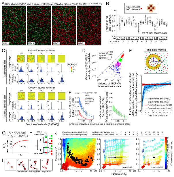
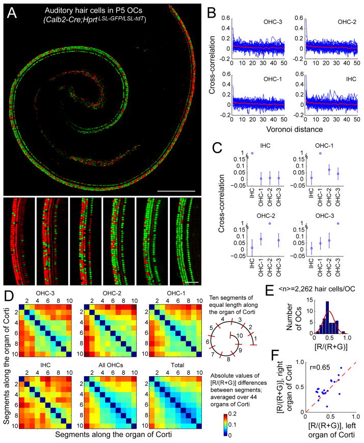
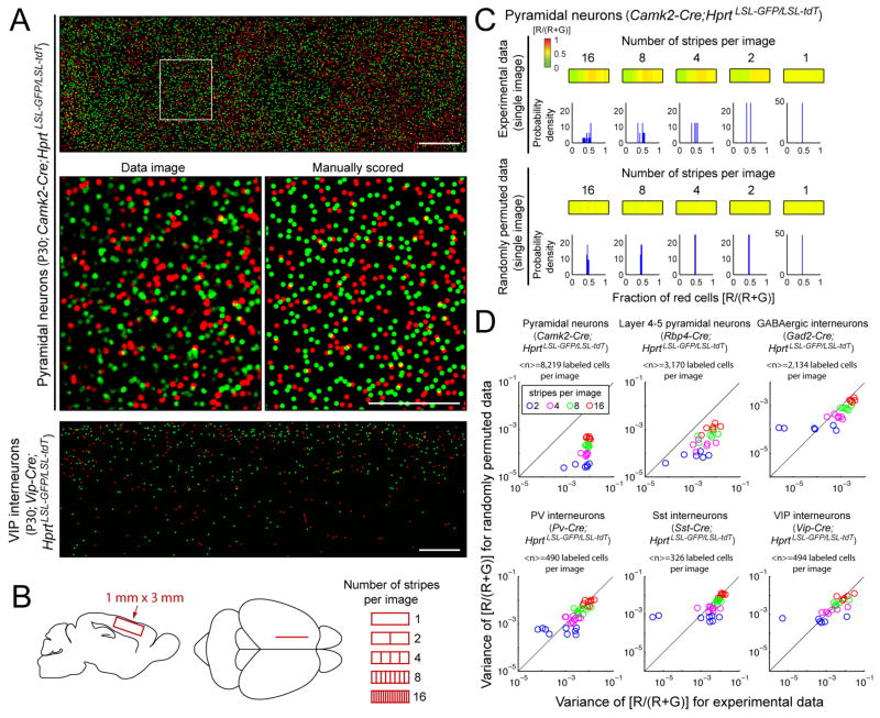
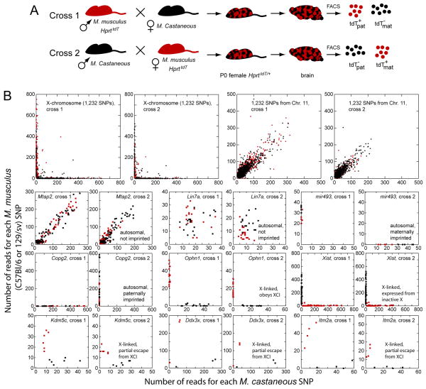
Female eutherian mammals use X chromosome inactivation (XCI) to epigenetically regulate gene expression from ∼4% of the genome. To quantitatively map the topography of XCI for defined cell types at single cell resolution, we have generated female mice that carry X-linked, Cre-activated, and nuclear-localized fluorescent reporters--GFP on one X chromosome and tdTomato on the other. Using these reporters in combination with different Cre drivers, we have defined the topographies of XCI mosaicism for multiple CNS cell types and of retinal vascular dysfunction in a model of Norrie disease. Depending on cell type, fluctuations in the XCI mosaic are observed over a wide range of spatial scales, from neighboring cells to left versus right sides of the body. These data imply a major role for XCI in generating female-specific, genetically directed, stochastic diversity in eutherian mammals on spatial scales that would be predicted to affect CNS function within and between individuals.

Figure 1. A dual-color genetic system for cell-type selective visualization of XCI mosaicism

(A) Diagram showing Cre activation of the two reporters at the X-linked Hprt locus. (B–R) Representative images showing XCI mosaicism in various tissues from females heterozygous for the Hprt reporters. In panels (F,G,K–M) the mice carry Hprt^{LSL-GFP/LSL-tdT} together with a tissue–specific Cre driver; all other panels are from Hprt^GFP/tdT mice. Scale bars: 50 um (P,R); 100 um (E,G,M,O,Q); 200 um (B–D,F,H–K); and 500 um (L,N). (S,T) Hprt^GFP/tdT females that are either siblings and half-siblings (S) or siblings (T) show variability in whole body [R/(R+G)] ratios. Stitching artifacts in the composite images account for minor intensity variation in a checkerboard pattern.

Figure 2. Quantitative analysis of XCI mosaicism among cone photoreceptors

(A) Cone photoreceptors in flat mounted retinas from four territories from a single Cone-Cre;Hprt^{LSL-GFP/LSL-tdT} mouse. L, left retina; R, right retina. Scale bar, 50 um. (B) Top, schematic showing the four territories imaged per retina. Bottom, [R/(R+G)] ratios for cones in each territory. Comparing the mean [R/(R+G)] ratios for left vs. right retinas, the correlation coefficient (r)=0.26. Bars, mean +/− S.D. (C–E) The square method. (C) Subdivision of each 640 × 640 um territory into the indicated number of squares; [R/(R+G)] histogram for a single territory and for all 88 territories. The smooth curve shows a Gaussian with mean=0.5 and variance matching each set of averaged data. Bottom, permuted control with cone locations unchanged but R vs. G identities randomly permuted. For probability density histograms, X-axis bin sizes are 0.02; the area under each curve is 1. (D) Variances of [R/(R+G)] for the experimental and randomly permuted data sets for each of the 88 territories with subdivisions at four spatial scales. (E) Left, means and standard deviations of the 88 variances of [R/(R+G)] for experimental and randomly permuted data sets. The subdivisions are (starting from the far right): 4 squares/image, 9 squares/image, 16 squares/image, etc. Right, the difference between the two curves. (F) The circle method. Top, schematic showing an annulus bounded by radii r₁ and r₂ and centered on one cone. For each cone, the fraction of the surrounding cells that differ in color from the central cell was determined for a contiguous series of annuli, and this value was normalized to the [R/(R+G)] ratio for that image. Bottom, blue lines, mean [R/(R+G)] (normalized to 1.0 for each territory) as a function of distance for all cones in each territory. Red lines, cone identities randomly permuted. (G–I) Modeling the development of the XCI mosaic with two degrees of freedom: number of founder cells and cell migration. (G) Circle method parameters D and X₀: for each cone, [R/(R+G)] asymptotically approaches a normalized value of 1.0, approximated by P/P₀=(1-De^−x/x0), where P₀=2P_tdTP_GFP is the value of P at infinite distance. X=Voronoi distance. (H) The lineage model: the vertical arrow indicates the founder pool. (I) The four steps for each round of cell division: (1) starting configuration, (2) randomly oriented cell division, (3) cell migration, and (4) cell positions adjusted to avoid crowding. (J) Comparison between observation and simulation. For each of the 88 images, simulations were performed with a [R/(R+G)] ratio in the progenitor pool that matched the observed ratio. The size of the simulated progenitor pool varied inversely with the number of cell divisions from founder cells to adult retina. 400 simulations were performed for each combination of founder cell number and migration rate, and the resulting mosaic of R and G cells was analyzed using the circle method to derive D and X₀ values. For each combination of founder cell number (symbol) and migration rate (color), the plots show individual D and X₀ values (left), mean and SD (center), and mean and SEM (right). Black dots, experimental data.

Figure 3. Regional and inter-individual variation in XCI mosaicism in the organ of Corti

(A) Examples of flat mounted P5 Calb2-Cre;Hprt^{LSL-GFP/LSL-tdT} OCs illustrating the extent of XCI variability within a single OC (upper) and among OCs (lower). Occasional unlabeled hair cells likely reflect variegation of the Cre driver. Scale bars, 300 um (upper) and 50 um (lower). (B) Cross-correlations for R vs. G identity within each of the four rows of hair cells determined with a one-dimensional version of the circle method, normalized for each row to the overall [R/(R+G)] ratio. Blue lines, cross-correlations for all hair cells in each of 44 P5 Calb2-Cre;Hprt^{LSL-GFP/LSL-tdT} OCs. Red line, mean for the 44 OCs. (C) Cross-correlations for R vs. G identity among nearest neighbors across adjacent rows of hair cells, normalized to the [R/(R+G)] ratios of the two rows being compared. A value of 0 represents no correlation; 1.0 represents perfect correlation. (D) Heatmaps quantifying pairwise differences in [R/(R+G)] ratio in 10% length intervals for hair cells from base to apex for the 44 OCs. (E) [R/(R+G)] ratios for hair cells from 44 P5 Calb2-Cre;Hprt^{LSL-GFP/LSL-tdT} OCs. Smooth line, best-fitting binomial distribution. (F) [R/(R+G)] ratios for hair cells from 21 pairs of left and right P5 Calb2-Cre;Hprt^{LSL-GFP/LSL-tdT} OCs.

Figure 4. Cell-type differences in XCI mosaicism in the cerebral cortex

(A) Pyramidal neurons (upper panels) and Vip-expressing interneurons (bottom panel) in 1 mm × 3 mm sagittal images of adult cerebral cortex. The inset in the upper panel is enlarged in the center left panel (“data image”); the manually scored version of the same image, in which each GFP+ or tdT+ nucleus is represented as a green or red disc, respectively, is at center right. Scale bars, 300 um. (B) Left, location of 1 mm × 3 mm sagittal images for cortical neuron quantification. Right, stripe method for dividing the images. (C) The stripe method for analyzing XCI mosaicism illustrated with a single 1 mm × 3 mm Camk2-Cre;Hprt^{LSL-GFP/LSL-tdT} image, subdivided along its long axis into the indicated number of stripes. Upper panels, experimental data; lower panels, a control in which G vs. R identities have been randomly permuted. For probability density histograms, X-axis bin sizes are 0.02; the area under each curve is 1. (D) Variances of the [R/(R+G)] distributions. Variance for experimental data vs. the mean variance for 1,000 random permutations of R and G identity within each image. Each point represents a single 1 mm × 3 mm image, divided into the indicated number of stripes.

Figure 5. XCI mosaicism in retinal vascular development and in a mouse model of the Norrie disease carrier state

(A–D) P2 and adult retina flat mounts. Heterogeneity is observed in [R/(R+G)] ratio in radial vessels (B) and in outer plexiform layer (OPL) capillaries (C,D). Scale bars, 200 um. (E,F) Quantification of [R/(R+G)] ratios in retinal vasculature for four mice (eight retinas) at P2, P5, P15, and adulthood. For P5 to adulthood, only vessels with >25 ECs were included. (G–J) P22 female Ndp^+/−;Hprt^tdT/+ retina flatmounts immunostained for PLVAP and claudin5; the Z-stack images encompass only the inner and outer plexiform layer capillary beds to avoid inhomogeneities from superficial veins and arteries. Retina #565 exhibits coarse-grained XCI mosaicism and multiple PLVAP+ territories. Retina #566 (from a different mouse) has a higher fraction of WT (tdT+) cells and finer-grained XCI mosaicism. Scale bar, 1 mm. (K,L) Images were reduced from ~4,200 × 4,000 pixels to 100 × 95 pixels (L). The tdT and PLVAP intensities from a single horizontal row of pixels [location marked by yellow dots in (G) and (I)] are plotted in (K). Scale bar in (L), 200 um. (M,N) tdT and PLVAP intensities from 100 × 95 pixel images. Compared to retina #566, retina #565 shows a broader distribution of tdT intensities (N, right two panels), implying more variability in the XCI mosaic at this spatial scale, and a broader range of PLVAP intensities (N, left two panels). tdT and PLVAP intensity distributions are anti-correlated (M). (O–Q) The 5.88 mm × 5.6 mm image of retina #565 was divided into squares of 280 um × 280 um, from which ten squares with average PLVAP intensities <20 and ten squares with PLVAP intensities >30 were selected at random. Panel (O) shows two examples of each category. Average tdT and PLVAP intensities for the 20 squares are plotted in (P) and (Q). The box and whisker plots in (Q) mark the median, the 25^th and 75^th percentiles, and the extremes. P value, non-paired student t-test. Scale bar in (O), 100 um.

Figure 6. Left-right asymmetry in XCI mosaicism

(A) E11.5 Hprt^tdT/GFP embryo, dorsal view of neural tube. Scale bar, 200 um. (B) Dorsal view and quantification of [G/(G+R)] pixel counts along the A-P axis for left and right sides of an E11.5 Hprt^tdT/GFP neural tube. Scale bar, 100 um. Anterior is at the left for (A) and (B). (C) Mean [G/(G+R)] pixel counts in left vs. right sides of 16 E11.5 neural tubes, as quantified in B. (D) Cross-correlations between [G/(G+R)] pixel counts along left vs. right sides of 16 E11.5 neural tubes (as shown in B); mean correlation is zero. Control comparisons are between images from the same side of the neural tube but differing in lateral position by 20%, 40%, and 60% of their widths or in depth by 6 um and 12 um. The high cross-correlation in the control comparisons imply that small changes in image location would have only a modest effect on the left-right cross-correlation. (E) XCI mosaicism among POMC neurons (left) and spinal motor neurons (right) in coronal sections of adult hypothalamus and spinal cord, respectively. Upper panels, representative sections. Lower panels, quantification of [R/(R+G)] ratios determined separately for left and right sides from 3–7 coronal sections for each of six mice. By convention, the side with the larger [R/(R+G)] ratio is plotted on the Y-axis. Scale bars, 200 um. (F) Variation in XCI mosaicism in left vs. right retinas in a single adult mouse. Scale bar, 500 um. (G) Variation in XCI topography in left and right eye-cups in three E11.5 embryos. Scale bar, 100 um. (H) XCI mosaicism in an adult brain shows left/right asymmetry among excitatory neurons in the cortex and hippocampus. In this Figure and in all other images of adult cells other than skeletal muscle, GFP and tdT expression is mutually exclusive. The rare nucleus that appears yellow reflects the superposition of two differently colored nuclei in different Z-planes. Scale bar, 1 mm.

Figure 7. RNAseq identifies genes subject to or partially escaping XCI in the early postnatal mouse brain

(A) Reciprocal crosses between M. musculus and M. castaneous. FACS purification of dissociated P0 brain cells from Hprt^tdT/+ female progeny: four populations were purified for RNAseq. Subscripts ‘pat’ or ‘mat’ refer, respectively, to the paternal or maternal origin of the Hprt^tdT allele. (B) Scatter plots showing the number of RNAseq reads per SNP from the four cell populations shown in (A). Each pair of adjacent scatter plots shows SNP data from cross 1 (left plot) and cross 2 (right plot). Red and black symbols represent reads from tdT+ and tdT- cells, respectively. Upper row, all X-chromosome SNPs (left) and an equal number of autosomal SNPs (right). Lower three rows, SNP data from nine genes illustrating the principal patterns of epigenetic regulation. In these plots, black symbols have been overlaid on red ones.

Figure 8. Model of stimulus-response characteristics for neural circuits in females homozygous or heterozygous for allelic variation

Left, squares represent individual neurons within a neural circuit, and red and green colors represent the gene products encoded by a pair of functionally distinct alleles. Right, stimulus-response properties for the neural circuit. A same dynamic range is predicted for the two classes of homozygotes (upper two panels) or, if the gene of interest resides on an autosome, for heterozygotes (third panel), because in each case the neural circuit is homogeneous with respect to production of the gene product of interest. However, if the gene of interest resides on the X-chromosome, a larger dynamic range is predicted for heterozygous females because XCI mosaicism would create a neural circuit that consists of two biochemically distinct classes of cells.

References

1. Amos-Landgraf JM, Cottle A, Plenge RM, Friez M, Schwartz CE, Longshore J, Willard HF. X chromosome-inactivation patterns of 1,005 phenotypically unaffected females. Am J Hum Genet. 2006;79:493–499. - PMC - PubMed
1. Berger W, Ropers HH. Norrie Disease. In: Scriver CR, Beaudet AL, Sly WS, Valle D, editors. Metabolic and Molecular Bases of Inherited Disease. 8. New York: McGraw Hill; 2001. pp. 5977–5985.
1. Carrel L, Willard HF. X-inactivation profile reveals extensive variability in X-linked gene expression in females. Nature. 2005;434:400–404. - PubMed
1. Cattanach BM. Control of chromosome inactivation. Annu Rev Genet. 1975;9:1–18. - PubMed
1. Chahrour M, Zoghbi HY. The story of Rett syndrome: from clinic to neurobiology. Neuron. 2007;56:422–437. - PubMed
Publication types