Mean-field models for heterogeneous networks of two-dimensional integrate and fire neurons

Abstract

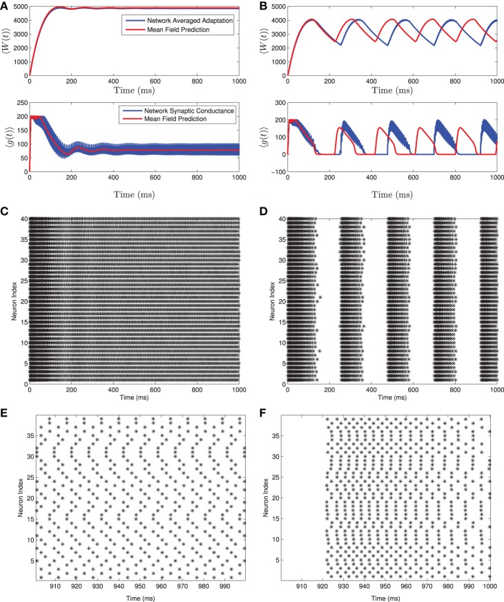
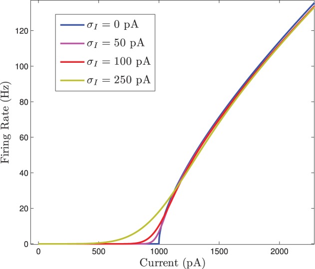
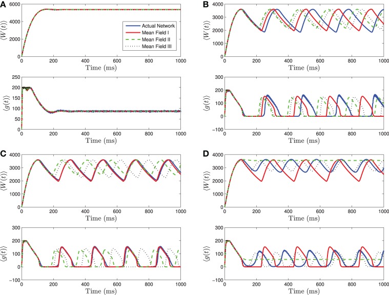
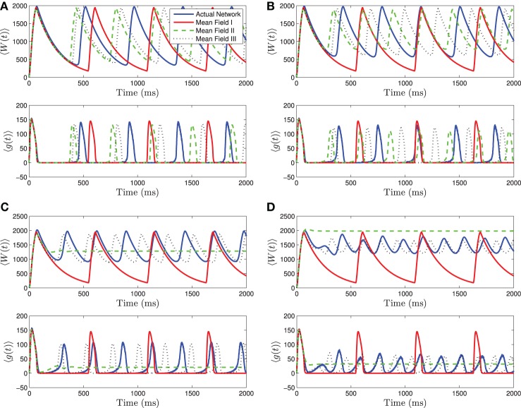
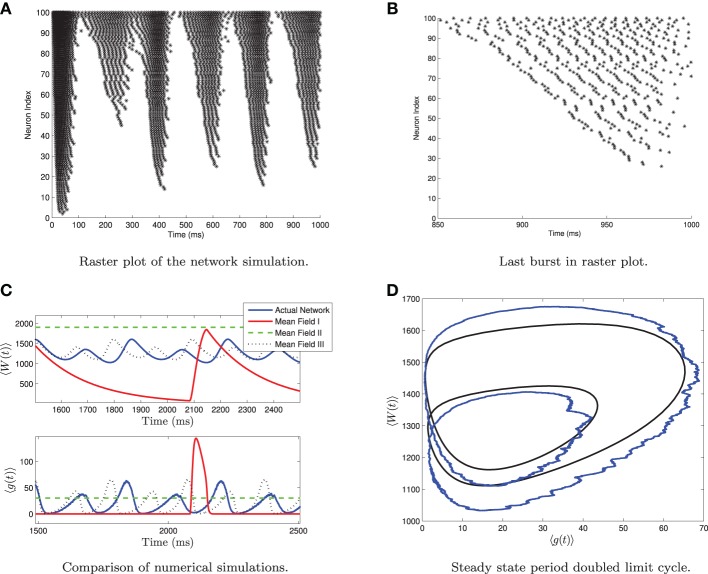
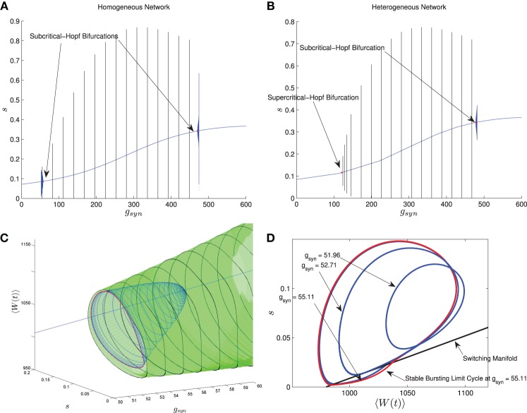
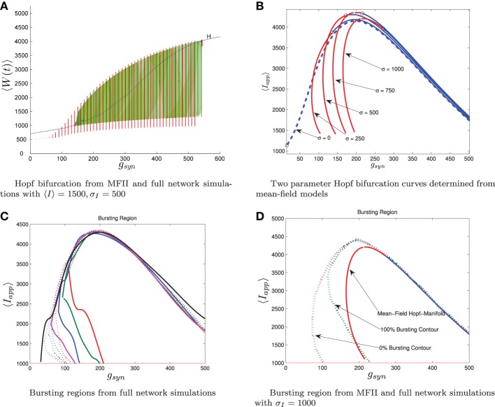
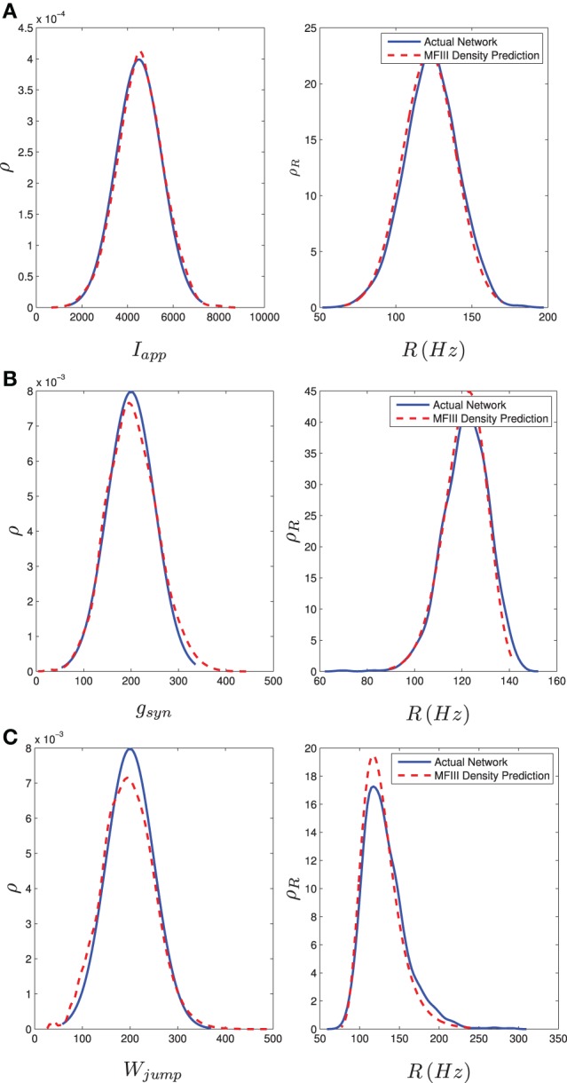
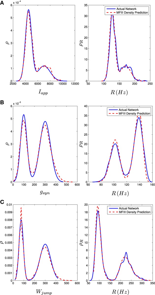
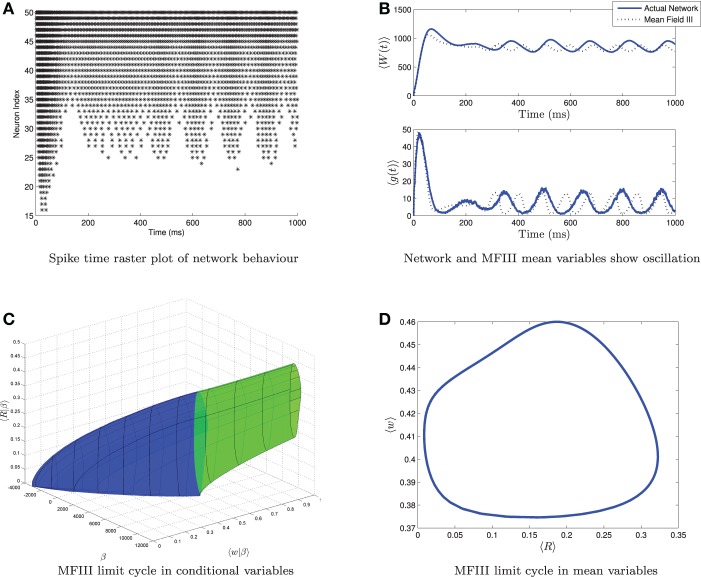
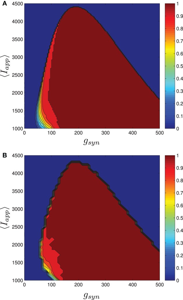
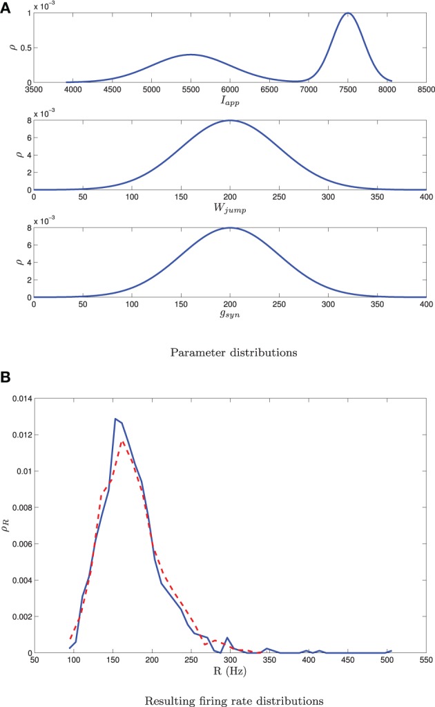
We analytically derive mean-field models for all-to-all coupled networks of heterogeneous, adapting, two-dimensional integrate and fire neurons. The class of models we consider includes the Izhikevich, adaptive exponential and quartic integrate and fire models. The heterogeneity in the parameters leads to different moment closure assumptions that can be made in the derivation of the mean-field model from the population density equation for the large network. Three different moment closure assumptions lead to three different mean-field systems. These systems can be used for distinct purposes such as bifurcation analysis of the large networks, prediction of steady state firing rate distributions, parameter estimation for actual neurons and faster exploration of the parameter space. We use the mean-field systems to analyze adaptation induced bursting under realistic sources of heterogeneity in multiple parameters. Our analysis demonstrates that the presence of heterogeneity causes the Hopf bifurcation associated with the emergence of bursting to change from sub-critical to super-critical. This is confirmed with numerical simulations of the full network for biologically reasonable parameter values. This change decreases the plausibility of adaptation being the cause of bursting in hippocampal area CA3, an area with a sizable population of heavily coupled, strongly adapting neurons.

Keywords: bifurcation analysis; bursting; hippocampus; integrate-and-fire neuron; mean-field model.

Figure 1

Numerical simulation of a homogeneous network of 1000 Izhikevich neurons, with parameters as follows. (A,C,E) I_app = 4500 pA, g_syn = 200 nS (B,D,F) I_app = 3500 pA, g_syn = 200 nS. The rest of the parameters can be found in Table 1. Simulations of the mean-field equations (in red) and the mean values of the corresponding full network simulations (in blue) showing (A) tonic firing and (B) bursting. In this and the following figures 〈W(t)〉 is the network mean adaptation variable in dimensional form and 〈g(t)〉 = g_syns(t) is the network mean synaptic conductance. (B,D) Raster plots for 40 randomly selected neurons from the network simulation in (A,C). (E,F) are the last 100 ms of the raster plots in (C,D), respectively. The mean-field equations are fairly accurate both when the network is tonically firing and when it is bursting. For the tonic firing case the neurons fire asynchronously at steady state, while in the bursting case, the neurons seem to align into two synchronously firing subpopulations firing out of phase with one another during the burst.

Figure 2

The firing rate curve F(I) for a Gaussian distributed background current in the 〈R_i(t)〉 response curve for the homogeneous network. The F(I) curves are plotted for increasing values of σ_I which smooths out the square root type non-smoothness at the onset of firing.

Figure 3

Numerical simulations of a network of 1000 Izhikevich neurons with parameters as in Table 1, except g_syn = 200 and the applied current which is normally distributed with mean and variance as follows. (A) 〈I_app〉 = 5000 pA, σ_I = 2000 pA. (B) 〈I_app〉 = 3000 pA, σ_I = 200 pA. (C) 〈I_app〉 = 3000 pA, σ_I = 500 pA. (D) 〈I_app〉 = 3000 pA, σ_I = 2000 pA. Blue is the network average of a given variable, red is MFI, green is MFII and black is MFIII. In this region, the mean-driving current is away from rheobase, 〈I_app〉 » I_rh. All three approximations are quantitatively and qualitatively similar for small to intermediate sized variances in the distribution of currents. For small variances, MFI is the most accurate and for larger variances, MFIII is the most accurate. For large variance, MFII bifurcates back to tonic firing earlier than MFI and MFIII, as seen in (D).

Figure 4

Numerical simulations of a network of 1000 neurons with parameters as in Table 1, except g_syn = 200 and the applied current which is normally distributed with mean and variance as follows. (A) 〈I_app〉 = 1200 pA, σ_I = 200 pA. (B) 〈I_app〉 = 1200 pA, σ_I = 500 pA. (C) 〈I_app〉 = 1200 pA, σ_I = 1000 pA. (D) 〈I_app〉 = 1200 pA, σ_I = 2000 pA. Blue is the network average of a given variable, red is MFI, green is MFII, and black is MFIII. In these simulations, the mean-driving current is close to (and over) the rheobase. In all cases, MFI is the least accurate. This is because it depends only on 〈I_app〉. When 〈I_app〉 = O(I_rh), even for small variance, many of the neurons have I < I_rh and may not spike at all. (A,B) For small values of σ_I, all three approximations are qualitatively and quantitatively accurate. (C,D) For larger variance, σ_I = O(I_rh), only MFIII is qualitatively and quantitatively accurate. In this case, MFII bifurcates early to tonic firing.

Figure 5

Period doubled limit cycle in the heterogeneous network and in MFIII. The network consists of 5000 neurons, with parameters as in Table 1, except g_syn = 200 and the applied current which is normally distributed with mean 〈I_app〉 = 1100 pA and variance σ_I = 2000 pA. (A) Raster plot of 100 randomly selected neurons of the network arranged in order of increasing current. Individual neuron behaviors include burst firing, alternate burst firing, tonic firing and quiescence. (B) Close-up of raster plot. The neurons appear to fire in “traveling waves” during a burst. (C) Comparison of the mean variables of the large network simulation and the simulations of the mean field systems. Only MFIII is able to reproduce the period doubling behavior. (D) Comparison of the “phase portrait” of period doubled limit cycle for MFIII and the mean variables of network.

Figure 6

Comparison between the bifurcation structure of homogeneous and heterogeneous networks using mean-field models. The parameters are as in Table 1, except the applied current which is normally distributed with mean and variance as follows and g_syn which varies as shown. (A) MFI, I_app = 2000 pA. (B) MFII, 〈I_app〉 = 2000 pA, σ_I = 500 pA. (C) MFI, low g_syn bifurcation sequence (3D view). (D) MFI, low g_syn bifurcation sequence, (2D view). In (A,B), the curved blue lines denote the value of the equilibrium point, which corresponds to tonic firing in the network. The vertical black/blue lines denote the amplitude range for the stable/unstable limit cycles, respectively. These correspond to bursting if the amplitude reaches zero, otherwise they correspond to the network having an oscillatory average firing rate. (A) Homogeneous case. Numerical bifurcation analysis of MFI displays two subcritical Hopf bifurcations: one at a low g_syn value and one at a high value. (B) Heterogeneous case. Numerical bifurcation analysis of MFII also displays two Hopf bifurcations, but the one at the low g_syn value is supercritical. This makes bursting at low g_syn values less robust in the heterogeneous case as discussed in the text. The non-smooth sequence of bifurcations for the homogeneous network is expanded upon in (C,D). In (C), we continue the smooth unstable limit cycle (blue) from the Hopf bifurcation at low g_syn values until the continuation halts (red). This occurs close to the grazing bifurcation with the switching manifold. We use direct numerical simulations to continue the stable non-smooth limit cycle (green). Key points in this bifurcation sequence are shown in the phase plane in (D). A smooth unstable limit cycle expands and grazes the switching manifold at approximately g_syn = 52.71 nS, and persists to collide in a non-smooth saddle-node of limit cycles at approximately g_syn = 55.11 nS. This sequence of bifurcations happens very rapidly in the parameter space, leaving a narrow region of bistability between the tonic firing and bursting solutions. Note that the totally unstable-non smooth limit cycles in (D) are computed via direct simulation of the time reversed MFII system.

Figure 7

Comparison between numerical bifurcation analysis of MFII and direct simulation of the full network. The parameters are as in Table 1, except g_syn varies as discussed below and the applied current which is normally distributed with mean and variance as discussed below. (A) Simulations of a network of 10,000 neurons with 〈I_app〉 and σ_I as shown were run at discrete values of g_syn for 2000 ms. The last 400 (ms) of simulation time is plotted (in red), showing the stable limit cycle oscillation for different g_syn values. This is compared to numerical continuation of the MFII limit cycle and equilibrium (in green and blue). Both the actual network and MFII appear to undergo a supercritical Hopf bifurcation for low g values and a subcritical Hopf for high g values. (B) The Hopf bifurcation curves for the mean-field systems with σ_I as shown. Red denotes supercritical Hopf bifurcations and blue denote subcritical Hopf bifurcations. The black circles denote codimension 2 Bautin bifurcation points. (C) Simulations of a network of 1000 neurons run on a discrete mesh of 〈I_app〉 and g_syn values. The 0% (dotted line) and 100% (solid line) network bursting contours for σ_I = 0, 250, 500, 750, and 1000 pA are colored in black, magenta, blue, green, and red, respectively. The curves are spline fits to the actual contours. (D) MFII Hopf bifurcation curves and spline fits to the 0% bursting and 100% bursting contours of the actual network for σ_I = 1000.

Figure 8

Heterogeneity in I_app, g_syn, or W_jump leads to heterogeneity in the firing rate. As described in section 3.2.2, given the parameter distribution (solid curves, left column) MFIII can be used to estimate the corresponding distribution of firing rates in the network (dashed curves, right column). As described in section 3.2.3, given the steady state firing rate distribution of an actual network (solid curves, right column) MFIII can be used to estimate the parameter distribution in the network (dashed curves, left column). The network firing rate distribution is estimated using a histogram. The calculations were carried out on a network of 1000 neurons. Parameters, other than those given below, can be found in Table 1. (A) Distribution of I_app with 〈I_app〉 = 4500 pA, σ_I = 1000 pA. (B) Distribution of g_syn with 〈g_syn〉 = 200 nS, σ_g = 50 nS. (C) Distribution of W_jump with 〈W_jump〉 = 200 pA, σ_W = 50 nS.

Figure 9

Bimodal distributions in I_app, g_syn, and W_jump lead to bimodal distributions in the firing rate. These bimodal parameter distributions are generated through distribution mixing of two normal subpopulations with standard deviations and means as given below. See Appendix C for details. The distribution of the firing rate or the distribution of the parameter can be computed using MFIII if one knows the complementary distribution. See sections 3.2.2 and 3.2.3 for details. Curve descriptions are as given in Figure 8. Parameters, other than those given below, can be found in Table 1. The calculations were carried out on a network of 1000 neurons. (A) Distribution of I_app with μ₁ = 4500 pA, σ₁ = 500 pA, μ₂ = 7000 pA, σ₂ = 1000 pA, m = 0.7. (B) Distribution of g_syn with μ₁ = 100 nS, σ₁ = 30 nS, μ₂ = 300 nS, σ₂ = 50 nS, m = 0.4. (C) Distribution of W_jump with μ₁ = 300 pA, σ₁ = 50 pA, μ₂ = 75 pA, σ₂ = 20 pA, m = 0.6.

Figure 10

Visualizing a limit cycle in a heterogeneous network. Numerical simulation of MFIII and a network of 1000 neurons with heterogeneity in the applied current. Parameters are as given in Table 1 except g_syn = 200 nS, 〈I_app〉 = 1000 pA and σ_I = 4400 pA. (A) Raster plot for 50 randomly selected neurons of the network arranged in order of increasing current. Some of the neurons are bursting, while others are tonically firing, albeit with an oscillatory firing rate. (B) In the mean variables, the steady state behavior of both the network and MFIII is an oscillation. (C) As MFIII is a partial differential equation, the steady state “limit cycle” is actually a manifold of limit cycles, foliated by the heterogeneous parameter β = I_app. Part of the manifold has cycles with 〈R|β〉 = 0 for an extended period of time (in blue). The other part contains limit cycles that have 〈R|β〉 ≠ 0 during the entire oscillation. We can classify neurons with the parameter values in blue as bursting, and those in green as oscillatory firing. (D) Averaging the limit cycle in (C) with respect to β yields the mean limit cycle.

Figure 11

The proportion of bursting neurons, p_burst for MFIII and an actual network. (A) Using the techniques outlined in the text, MFIII is used to compute the proportion of bursting neurons, p_burst at each point in a mesh over the parameter space. (B) Numerical simulations of a network of 500 neurons are used to compute the proportion of bursting neurons, p_burst. All the parameters for both the MFIII system and the actual network are identical (see Table 1), except that MFIII is run over a finer mesh. The results using MFIII are both qualitatively and quantitatively accurate. (A) MFIII, σ_I = 500 pA. (B) Network, σ_I = 500 pA.

Figure 12

A bimodal distribution in I_app together with unimodal distributions in g_syn and W_jump as shown in (A) yields a unimodal distribution in the firing rate [dashed curve in (B)]. The mean-field equations give a good estimate of this distribution [solid curve in (B)]. Simulations are for network of 1000 neurons. parameter given in Table 1 except I, g, and W_jump. These are distributed with σ_w = 50, 〈W_jump〉 = 200, σ_g = 50, 〈g_syn〉 = 200, m = 0.5, 〈I_{app, 1}〉 = 7500, σ_{I, 1} = 200, 〈I_{app, 2}〉 = 5500, σ_{I, 2} = 500. Other combinations of bimodal and unimodal parameter distributions may yield bimodal firing rate distributions. Note that this is different than the situation shown in Figure 9, where a single bimodal source of heterogeneity yielded a bimodal firing rate distribution.

Figure 13

Case study: the proportion of bursting neurons in a network with both strongly adapting and weakly adapting neurons. Parameters are as in Table 1 except the I_app, g_syn, W_jump, and τ_W which have bimodal distributions generated by distribution mixing with parameters given in Table 2. The parameter p_SA represents the proportion of strongly adapting neurons in the network (see Equation A8). The dashed line is the 0% bursting contour, while the dotted line is the 100% bursting contour. As shown in both the network (A) and MFIII (B), the bursting regions becomes significantly smaller when the proportion of strongly adapting neurons decreases. In all cases, the curves are smoother spline fits to the actual contours.

References

1. Abbott L. F., van Vreeswijk C. (1993). Asynchronous states in networks of pulse-coupled oscillators. Learn Mem. 48, 1483–1490 - PubMed
1. Andersen P., Morris R., Amaral D., Bliss T., O'Keefe J. (eds.). (2006). The Hippocampus Book. Oxford: Oxford University Press
1. Bressloff P. C. (2012). Spatiotemporal dynamics of continuum neural fields. J. Phys. A. Math. Theor. 45:033001 10.1088/1751-8113/45/3/033001 - DOI - PubMed
1. Brette R., Gerstner W. (2005). Adaptive exponential integrate-and-fire model as an effective description of neuronal activity. J. Neurophys. 94, 3637–3642 10.1152/jn.00686.2005 - DOI - PubMed
1. Buzsáaki G. (2004). Large-scale recordings of neuronal ensembles. Nat. Neurosci. 7, 446–451 10.1038/nn1233 - DOI - PubMed
LinkOut - more resources