. 2014 Jan-Feb;34(1):4-17.
doi: 10.1148/rg.341135038.

Emerging techniques for dose optimization in abdominal CT

Affiliations

Emerging techniques for dose optimization in abdominal CT

Ravi K Kaza et al. Radiographics. 2014 Jan-Feb.

Abstract

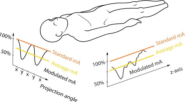
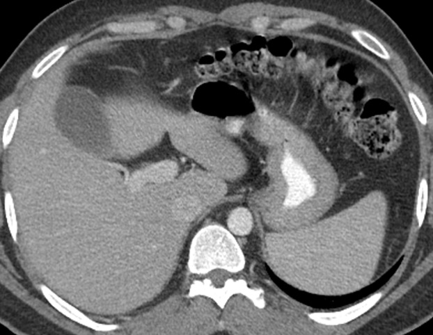
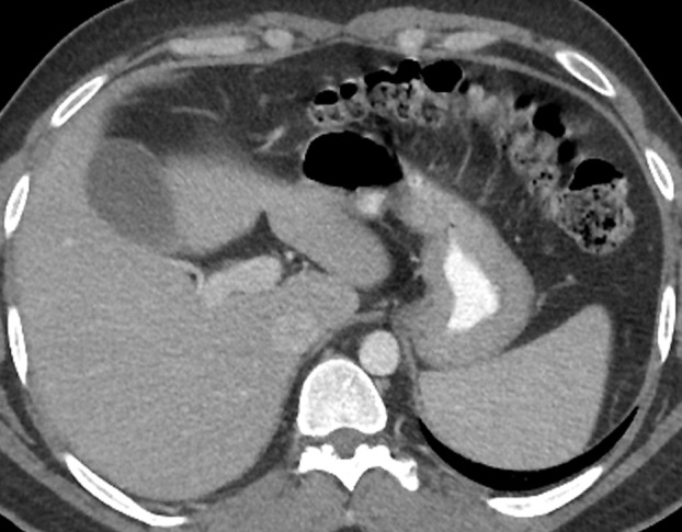
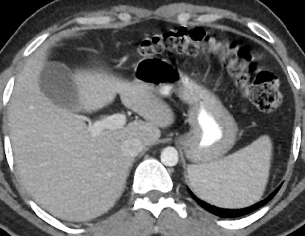
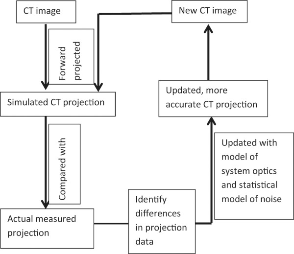
Recent advances in computed tomographic (CT) scanning technique such as automated tube current modulation (ATCM), optimized x-ray tube voltage, and better use of iterative image reconstruction have allowed maintenance of good CT image quality with reduced radiation dose. ATCM varies the tube current during scanning to account for differences in patient attenuation, ensuring a more homogeneous image quality, although selection of the appropriate image quality parameter is essential for achieving optimal dose reduction. Reducing the x-ray tube voltage is best suited for evaluating iodinated structures, since the effective energy of the x-ray beam will be closer to the k-edge of iodine, resulting in a higher attenuation for the iodine. The optimal kilovoltage for a CT study should be chosen on the basis of imaging task and patient habitus. The aim of iterative image reconstruction is to identify factors that contribute to noise on CT images with use of statistical models of noise (statistical iterative reconstruction) and selective removal of noise to improve image quality. The degree of noise suppression achieved with statistical iterative reconstruction can be customized to minimize the effect of altered image quality on CT images. Unlike with statistical iterative reconstruction, model-based iterative reconstruction algorithms model both the statistical noise and the physical acquisition process, allowing CT to be performed with further reduction in radiation dose without an increase in image noise or loss of spatial resolution. Understanding these recently developed scanning techniques is essential for optimization of imaging protocols designed to achieve the desired image quality with a reduced dose.


Figures

Figure 1
Figure 1
Drawing illustrates the modulation of tube current (in milliamperes [mA]) along the longitudinal (z) and horizontal (x-y) axes of the patient.
Figure 2a
Figure 2a
Axial 5-mm-thick reconstructed image from a CT study performed with a noise index of 35 at 2.5-mm thickness (a) shows increased noise compared with the corresponding image from a prior study performed with a noise index of 22 at the same thickness (b). The CT dose index volume (CTDIvol) values were 1.88 and 4.67 mGy, respectively.
Figure 2b
Figure 2b
Axial 5-mm-thick reconstructed image from a CT study performed with a noise index of 35 at 2.5-mm thickness (a) shows increased noise compared with the corresponding image from a prior study performed with a noise index of 22 at the same thickness (b). The CT dose index volume (CTDIvol) values were 1.88 and 4.67 mGy, respectively.
Figure 3a
Figure 3a
(a) Axial 0.625-mm-thick reconstructed image from a CT study performed with a noise index of 30 at 0.625-mm thickness demonstrates significant noise. (b) Axial 5-mm-thick reconstructed image from the same study shows reduced noise and improved image quality.
Figure 3b
Figure 3b
(a) Axial 0.625-mm-thick reconstructed image from a CT study performed with a noise index of 30 at 0.625-mm thickness demonstrates significant noise. (b) Axial 5-mm-thick reconstructed image from the same study shows reduced noise and improved image quality.
Figure 4a
Figure 4a
(a) Axial 5-mm-thick reconstructed image from a CT study that was performed with a noise index of 30 at 0.625-mm thickness. (b) Axial 5-mm-thick reconstructed image from a CT study performed with the same noise index in a different patient with more intraabdominal fat shows improved image quality compared with a.
Figure 4b
Figure 4b
(a) Axial 5-mm-thick reconstructed image from a CT study that was performed with a noise index of 30 at 0.625-mm thickness. (b) Axial 5-mm-thick reconstructed image from a CT study performed with the same noise index in a different patient with more intraabdominal fat shows improved image quality compared with a.
Figure 5a
Figure 5a
CT angiographic images (0.625-mm thickness) obtained with noise indices of 60 (a) and 30 (b) clearly depict a high-contrast endoleak (arrow). CTDIvol values were 2.76 and 14.24 mGy, respectively.
Figure 5b
Figure 5b
CT angiographic images (0.625-mm thickness) obtained with noise indices of 60 (a) and 30 (b) clearly depict a high-contrast endoleak (arrow). CTDIvol values were 2.76 and 14.24 mGy, respectively.
Figure 6
Figure 6
CT scout image with a grid overlay helps confirm that the patient is properly centered.
Figure 7a
Figure 7a
CT images obtained at 80 kV (a) and 120 kV (b) in a patient with Crohn disease show that, despite the increased noise, the 80-kV image demonstrates a better CNR and allows clearer visualization of the enhancing bowel wall (arrows).
Figure 7b
Figure 7b
CT images obtained at 80 kV (a) and 120 kV (b) in a patient with Crohn disease show that, despite the increased noise, the 80-kV image demonstrates a better CNR and allows clearer visualization of the enhancing bowel wall (arrows).
Figure 8a
Figure 8a
Abdominal CT images obtained at 80 kV viewed at a typical window width and level of 400/40 (a) and an optimized window width and level of 950/150 (b) show how the use of increased window width and level when viewing an image obtained at low-kilovolt scanning reduces perceived image noise, with resultant perceived improvement of image quality.
Figure 8b
Figure 8b
Abdominal CT images obtained at 80 kV viewed at a typical window width and level of 400/40 (a) and an optimized window width and level of 950/150 (b) show how the use of increased window width and level when viewing an image obtained at low-kilovolt scanning reduces perceived image noise, with resultant perceived improvement of image quality.
Figure 9a
Figure 9a
Pseudoenhancement in a renal cyst. (a) CT image obtained at 120 kV shows a lesion in the kidney with a measured attenuation of about 18 HU. (b) On a subsequent CT image obtained at 80 kV, the lesion has an attenuation of nearly 60 HU. The lesion was confirmed to be a simple cyst at MR imaging.
Figure 9b
Figure 9b
Pseudoenhancement in a renal cyst. (a) CT image obtained at 120 kV shows a lesion in the kidney with a measured attenuation of about 18 HU. (b) On a subsequent CT image obtained at 80 kV, the lesion has an attenuation of nearly 60 HU. The lesion was confirmed to be a simple cyst at MR imaging.
Figure 10a
Figure 10a
Axial CT images (0.625-mm thickness) reconstructed with filtered back projection (FBP) reconstruction (a), 30% ASIR (b), 70% ASIR (c), and 100% ASIR (d).
Figure 10b
Figure 10b
Axial CT images (0.625-mm thickness) reconstructed with filtered back projection (FBP) reconstruction (a), 30% ASIR (b), 70% ASIR (c), and 100% ASIR (d).
Figure 10c
Figure 10c
Axial CT images (0.625-mm thickness) reconstructed with filtered back projection (FBP) reconstruction (a), 30% ASIR (b), 70% ASIR (c), and 100% ASIR (d).
Figure 10d
Figure 10d
Axial CT images (0.625-mm thickness) reconstructed with filtered back projection (FBP) reconstruction (a), 30% ASIR (b), 70% ASIR (c), and 100% ASIR (d).
Figure 11
Figure 11
Diagram of the steps of iterative reconstruction. With each successive iteration, the difference between the simulated and measured projection is reduced. The iterative process is usually discontinued when the predefined image quality criterion is met.
Figure 12a
Figure 12a
CT images obtained at a fixed tube current with FBP reconstruction (a) and with ATCM at a noise index of 30 at 0.625-mm thickness with 30% ASIR reconstruction (b) show similar image noise and quality. CTDIvol values were 21.3 and 12.3 mGy, respectively.
Figure 12b
Figure 12b
CT images obtained at a fixed tube current with FBP reconstruction (a) and with ATCM at a noise index of 30 at 0.625-mm thickness with 30% ASIR reconstruction (b) show similar image noise and quality. CTDIvol values were 21.3 and 12.3 mGy, respectively.
Figure 13
Figure 13
Drawing illustrates CT projection acquisition. The entire projection is represented as multiple pencil beams for FBP image reconstruction, one of which is shown as a single line. MBIR allows more comprehensive 3D modeling of x-ray generation from the focal spot, interaction with the patient, and capture at the detectors (shaded area).
Figure 14a
Figure 14a
Axial 0.625-mm-thick images from a low-dose CT study (CTDIvol = 2.5 mGy, effective dose = 1.8 mSv) reconstructed with FBP (a), 50% ASIR (b), 100% ASIR (c), and MBIR (d) show a progressive decrease in image noise. Two small hypoattenuating splenic lesions are seen on the MBIR image (arrows in d) that are not easily seen with FBP reconstruction or ASIR.
Figure 14b
Figure 14b
Axial 0.625-mm-thick images from a low-dose CT study (CTDIvol = 2.5 mGy, effective dose = 1.8 mSv) reconstructed with FBP (a), 50% ASIR (b), 100% ASIR (c), and MBIR (d) show a progressive decrease in image noise. Two small hypoattenuating splenic lesions are seen on the MBIR image (arrows in d) that are not easily seen with FBP reconstruction or ASIR.
Figure 14c
Figure 14c
Axial 0.625-mm-thick images from a low-dose CT study (CTDIvol = 2.5 mGy, effective dose = 1.8 mSv) reconstructed with FBP (a), 50% ASIR (b), 100% ASIR (c), and MBIR (d) show a progressive decrease in image noise. Two small hypoattenuating splenic lesions are seen on the MBIR image (arrows in d) that are not easily seen with FBP reconstruction or ASIR.
Figure 14d
Figure 14d
Axial 0.625-mm-thick images from a low-dose CT study (CTDIvol = 2.5 mGy, effective dose = 1.8 mSv) reconstructed with FBP (a), 50% ASIR (b), 100% ASIR (c), and MBIR (d) show a progressive decrease in image noise. Two small hypoattenuating splenic lesions are seen on the MBIR image (arrows in d) that are not easily seen with FBP reconstruction or ASIR.
Figure 15a
Figure 15a
(a, b) Axial 2.5-mm-thick (a) and coronal 2-mm-thick (b) MBIR images from low-dose CT enterography performed in a patient with Crohn disease at 80 kV with a noise index of 60 at 0.625-mm thickness (CTDIvol value = 1.9 mGy) show wall thickening and enhancement involving the neoterminal ileum (arrow in a). (c, d) Corresponding 30% ASIR images from an earlier standard-dose CT enterographic study performed in the same patient at 120 kV with a noise index of 30 at 0.625-mm thickness (CTDIvol value = 7.9 mGy) show similar findings (arrow in c).
Figure 15b
Figure 15b
(a, b) Axial 2.5-mm-thick (a) and coronal 2-mm-thick (b) MBIR images from low-dose CT enterography performed in a patient with Crohn disease at 80 kV with a noise index of 60 at 0.625-mm thickness (CTDIvol value = 1.9 mGy) show wall thickening and enhancement involving the neoterminal ileum (arrow in a). (c, d) Corresponding 30% ASIR images from an earlier standard-dose CT enterographic study performed in the same patient at 120 kV with a noise index of 30 at 0.625-mm thickness (CTDIvol value = 7.9 mGy) show similar findings (arrow in c).
Figure 15c
Figure 15c
(a, b) Axial 2.5-mm-thick (a) and coronal 2-mm-thick (b) MBIR images from low-dose CT enterography performed in a patient with Crohn disease at 80 kV with a noise index of 60 at 0.625-mm thickness (CTDIvol value = 1.9 mGy) show wall thickening and enhancement involving the neoterminal ileum (arrow in a). (c, d) Corresponding 30% ASIR images from an earlier standard-dose CT enterographic study performed in the same patient at 120 kV with a noise index of 30 at 0.625-mm thickness (CTDIvol value = 7.9 mGy) show similar findings (arrow in c).
Figure 15d
Figure 15d
(a, b) Axial 2.5-mm-thick (a) and coronal 2-mm-thick (b) MBIR images from low-dose CT enterography performed in a patient with Crohn disease at 80 kV with a noise index of 60 at 0.625-mm thickness (CTDIvol value = 1.9 mGy) show wall thickening and enhancement involving the neoterminal ileum (arrow in a). (c, d) Corresponding 30% ASIR images from an earlier standard-dose CT enterographic study performed in the same patient at 120 kV with a noise index of 30 at 0.625-mm thickness (CTDIvol value = 7.9 mGy) show similar findings (arrow in c).
Figure 16a
Figure 16a
(a, b) Axial 1.25-mm-thick images from a CT study performed at 120 kV and 80 mA that were reconstructed with ASIR (a) and MBIR (b) show a 2-mm calculus in the left kidney (arrow). CTDIvol = 3.57 mGy. (c, d) On axial 1.25-mm-thick images from a repeat low-dose CT study performed at 120 kV and 20 mA, the calculus is not well seen on the image reconstructed with ASIR due to increased image noise (arrow in c), but it is easily seen on the image reconstructed with MBIR due to better noise reduction (arrow in d). CTDIvol = 0.9 mGy.
Figure 16b
Figure 16b
(a, b) Axial 1.25-mm-thick images from a CT study performed at 120 kV and 80 mA that were reconstructed with ASIR (a) and MBIR (b) show a 2-mm calculus in the left kidney (arrow). CTDIvol = 3.57 mGy. (c, d) On axial 1.25-mm-thick images from a repeat low-dose CT study performed at 120 kV and 20 mA, the calculus is not well seen on the image reconstructed with ASIR due to increased image noise (arrow in c), but it is easily seen on the image reconstructed with MBIR due to better noise reduction (arrow in d). CTDIvol = 0.9 mGy.
Figure 16c
Figure 16c
(a, b) Axial 1.25-mm-thick images from a CT study performed at 120 kV and 80 mA that were reconstructed with ASIR (a) and MBIR (b) show a 2-mm calculus in the left kidney (arrow). CTDIvol = 3.57 mGy. (c, d) On axial 1.25-mm-thick images from a repeat low-dose CT study performed at 120 kV and 20 mA, the calculus is not well seen on the image reconstructed with ASIR due to increased image noise (arrow in c), but it is easily seen on the image reconstructed with MBIR due to better noise reduction (arrow in d). CTDIvol = 0.9 mGy.
Figure 16d
Figure 16d
(a, b) Axial 1.25-mm-thick images from a CT study performed at 120 kV and 80 mA that were reconstructed with ASIR (a) and MBIR (b) show a 2-mm calculus in the left kidney (arrow). CTDIvol = 3.57 mGy. (c, d) On axial 1.25-mm-thick images from a repeat low-dose CT study performed at 120 kV and 20 mA, the calculus is not well seen on the image reconstructed with ASIR due to increased image noise (arrow in c), but it is easily seen on the image reconstructed with MBIR due to better noise reduction (arrow in d). CTDIvol = 0.9 mGy.

Comment in

  • Invited commentary.
    Mahesh M. Mahesh M. Radiographics. 2014 Jan-Feb;34(1):17-8. doi: 10.1148/rg.341135177. Radiographics. 2014. PMID: 24428278 No abstract available.

Similar articles

Cited by

References

    1. McCollough CH, Guimarães L, Fletcher JG. In defense of body CT. AJR Am J Roentgenol. 2009;193(1):28–39. - PMC - PubMed
    1. Sodickson A, Baeyens PF, Andriole KP, et al. Recurrent CT, cumulative radiation exposure, and associated radiation-induced cancer risks from CT of adults. Radiology. 2009;251(1):175–184. - PubMed
    1. Health Physics Society. Radiation risk in perspective: position statement of the Health Physics Society. http://www.hps.org/documents/radiationrisk.pdf. Revised August 2004. Accessed May 20, 2013.
    1. Mettler FA, Jr, Bhargavan M, Faulkner K, et al. Radiologic and nuclear medicine studies in the United States and worldwide: frequency, radiation dose, and comparison with other radiation sources—1950–2007. Radiology. 2009;253(2):520–531. - PubMed
    1. McCollough CH, Primak AN, Braun N, Kofler J, Yu L, Christner J. Strategies for reducing radiation dose in CT. Radiol Clin North Am. 2009;47(1):27–40. - PMC - PubMed

Publication types