

VBA: a probabilistic treatment of nonlinear models for neurobiological and behavioural data
- PMID: 24465198
- PMCID: PMC3900378
- DOI: 10.1371/journal.pcbi.1003441
VBA: a probabilistic treatment of nonlinear models for neurobiological and behavioural data
Abstract
This work is in line with an on-going effort tending toward a computational (quantitative and refutable) understanding of human neuro-cognitive processes. Many sophisticated models for behavioural and neurobiological data have flourished during the past decade. Most of these models are partly unspecified (i.e. they have unknown parameters) and nonlinear. This makes them difficult to peer with a formal statistical data analysis framework. In turn, this compromises the reproducibility of model-based empirical studies. This work exposes a software toolbox that provides generic, efficient and robust probabilistic solutions to the three problems of model-based analysis of empirical data: (i) data simulation, (ii) parameter estimation/model selection, and (iii) experimental design optimization.
Conflict of interest statement
The authors have declared that no competing interests exist.
Figures

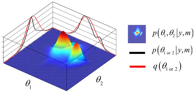
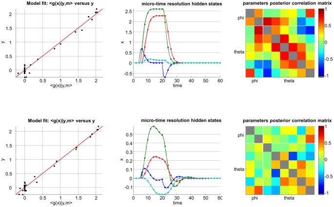
 . Here, the 2D landscape depicts a (true) joint posterior density
  and the two black lines are the subsequent marginal posterior densities of
  and
and  , respectively. The mean-field approximation basically describes the joint posterior density as the product of the two marginal densities (black profiles). In turn, stochastic dependencies between parameter subsets are replaced by deterministic dependencies between their posterior sufficient statistics. The Laplace approximation further assumes that the marginal densities can be described by Gaussian densities (red profiles).
 (blue) and
  (green) are plotted as a function of data y, given an arbitrary design u. The dashed grey line shows the marginal predictive density
  that captures the probabilistic prediction of the whole comparison set
  . The area under the curve (red) measures the model selection error rate
  , which depends upon the discriminability between the two prior predictive density
  and
and  . This is precisely what the Laplace-Chernoff risk
  is a measure of. Adapted from .

 and
and  ) given fMRI data time series. In this case, the problem reduces to deciding whether or not to introduce the second experimental factor (here,
  = attentional modulation), on top of the first factor (
 = photic stimulation). Upper left: the two network models to be compared given fMRI data (top/bottom: with/without attentional modulation of the V1→V5 connection). Upper middle: block-by-block temporal dynamics of design efficiency of both types of blocks. Green (resp. blue) dots correspond to blocks with (resp. without.) attentional modulation. Upper right: scan-by-scan temporal dynamics of the optimized (on-line) design. Lower left: scan-by-scan temporal dynamics of the simulated fMRI signal (blue: V1, green: V5). Lower middle: block-by-block temporal dynamics of 95% posterior confidence intervals on the estimated modulatory effect (under model
  ). The green line depicts the strength of the simulated effect. Lower right: block-by-block temporal dynamics of log Bayes factors
  .
.

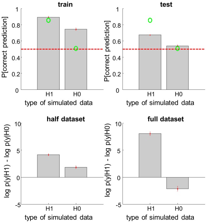
 , given the training dataset. Lower right: same format, given the full (train+test) dataset.
 .
.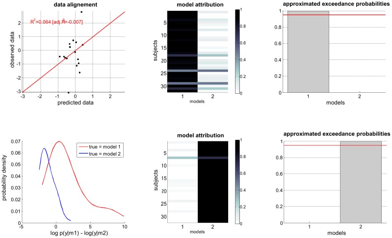
 , group 1) or a ‘reduced’ (
 , group 2) model. Upper left: simulated data (y-axis) plotted against fitted data (x-axis), for a typical simulation. Lower left: histograms of log Bayes factor
  , for both groups (red: group 1, blue: group 2). Upper middle: model attributions, for group 1. The posterior probability
  for each subject is coded on a black-and-white colour scale (black = 1, white = 0). Lower middle: same format, group 2. Upper right: exceedance probabilities, for group 1. The red line indicates the usual 95% threshold. Lower right: same format, group 2.
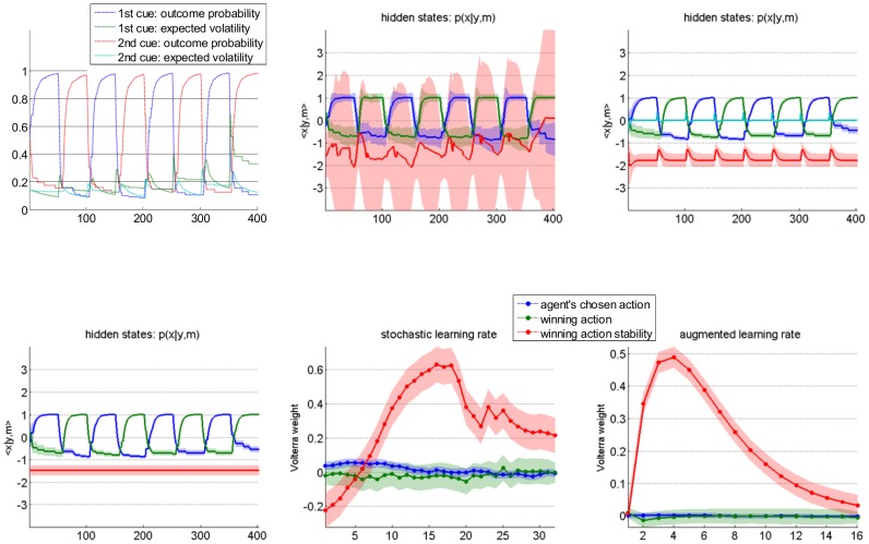
Similar articles
-
Automated parameter estimation for biological models using Bayesian statistical model checking.BMC Bioinformatics. 2015;16 Suppl 17(Suppl 17):S8. doi: 10.1186/1471-2105-16-S17-S8. Epub 2015 Dec 7. BMC Bioinformatics. 2015. PMID: 26679759 Free PMC article.
-
Globally multimodal problem optimization via an estimation of distribution algorithm based on unsupervised learning of Bayesian networks.Evol Comput. 2005 Spring;13(1):43-66. doi: 10.1162/1063656053583432. Evol Comput. 2005. PMID: 15901426
-
Goal-directed decision making as probabilistic inference: a computational framework and potential neural correlates.Psychol Rev. 2012 Jan;119(1):120-54. doi: 10.1037/a0026435. Psychol Rev. 2012. PMID: 22229491 Free PMC article.
-
Global optimization in systems biology: stochastic methods and their applications.Adv Exp Med Biol. 2012;736:409-24. doi: 10.1007/978-1-4419-7210-1_24. Adv Exp Med Biol. 2012. PMID: 22161343
-
Probabilistic inference in general graphical models through sampling in stochastic networks of spiking neurons.PLoS Comput Biol. 2011 Dec;7(12):e1002294. doi: 10.1371/journal.pcbi.1002294. Epub 2011 Dec 15. PLoS Comput Biol. 2011. PMID: 22219717 Free PMC article.
Cited by
-
The virtual loss function in the summary perception of motion and its limited adjustability.J Vis. 2021 May 3;21(5):2. doi: 10.1167/jov.21.5.2. J Vis. 2021. PMID: 33944907 Free PMC article.
-
Comparing continual task learning in minds and machines.Proc Natl Acad Sci U S A. 2018 Oct 30;115(44):E10313-E10322. doi: 10.1073/pnas.1800755115. Epub 2018 Oct 15. Proc Natl Acad Sci U S A. 2018. PMID: 30322916 Free PMC article.
-
Mood fluctuations shift cost-benefit tradeoffs in economic decisions.Sci Rep. 2023 Oct 24;13(1):18173. doi: 10.1038/s41598-023-45217-w. Sci Rep. 2023. PMID: 37875525 Free PMC article.
-
Neuro-computational account of how mood fluctuations arise and affect decision making.Nat Commun. 2018 Apr 26;9(1):1708. doi: 10.1038/s41467-018-03774-z. Nat Commun. 2018. PMID: 29700303 Free PMC article.
-
Contextual modulation of value signals in reward and punishment learning.Nat Commun. 2015 Aug 25;6:8096. doi: 10.1038/ncomms9096. Nat Commun. 2015. PMID: 26302782 Free PMC article.
References
-
- Schmidt A, Smieskova R, Aston J, Simon A, Allen P, et al.. (2013) Brain connectivity abnormalities predating the onset of psychosis: correlation with the effect of medication. JAMA Psychiatry 70(9): 903–12. - PubMed
-
- Daunizeau J, David O, Stephan KE (2011) Dynamic causal modeling: a critical review of the biophysical and statistical foundations. NeuroImage 58(2): 312–22. - PubMed
Publication types
MeSH terms
LinkOut - more resources
Full Text Sources
Other Literature Sources
Medical
Miscellaneous
