Development of ultra-high-density screening tools for microbial "omics"

Abstract

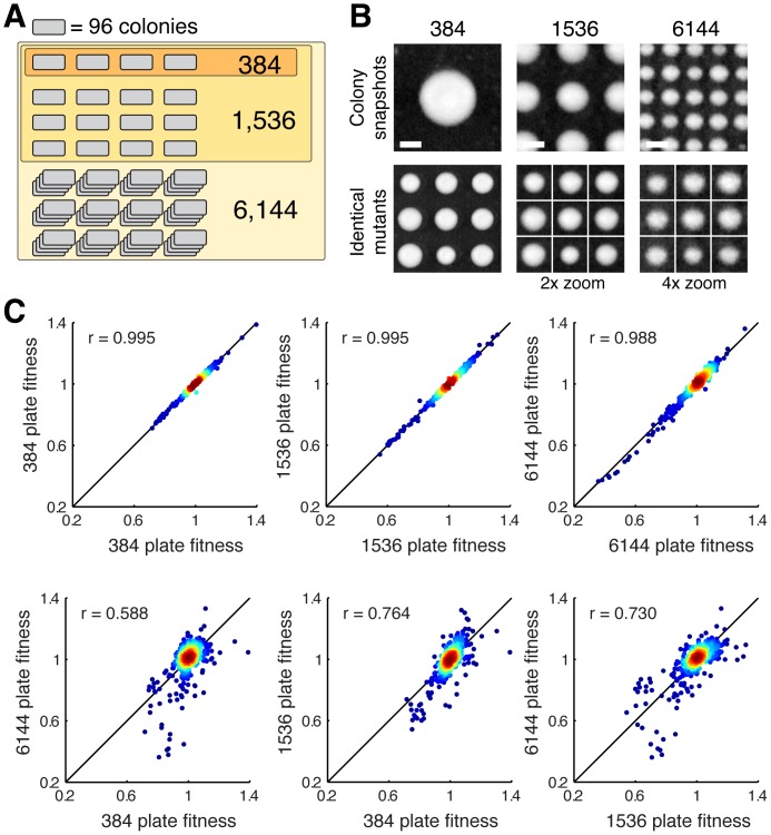
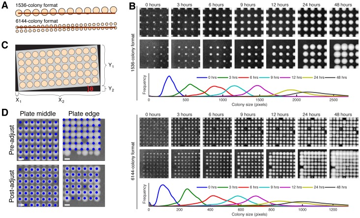
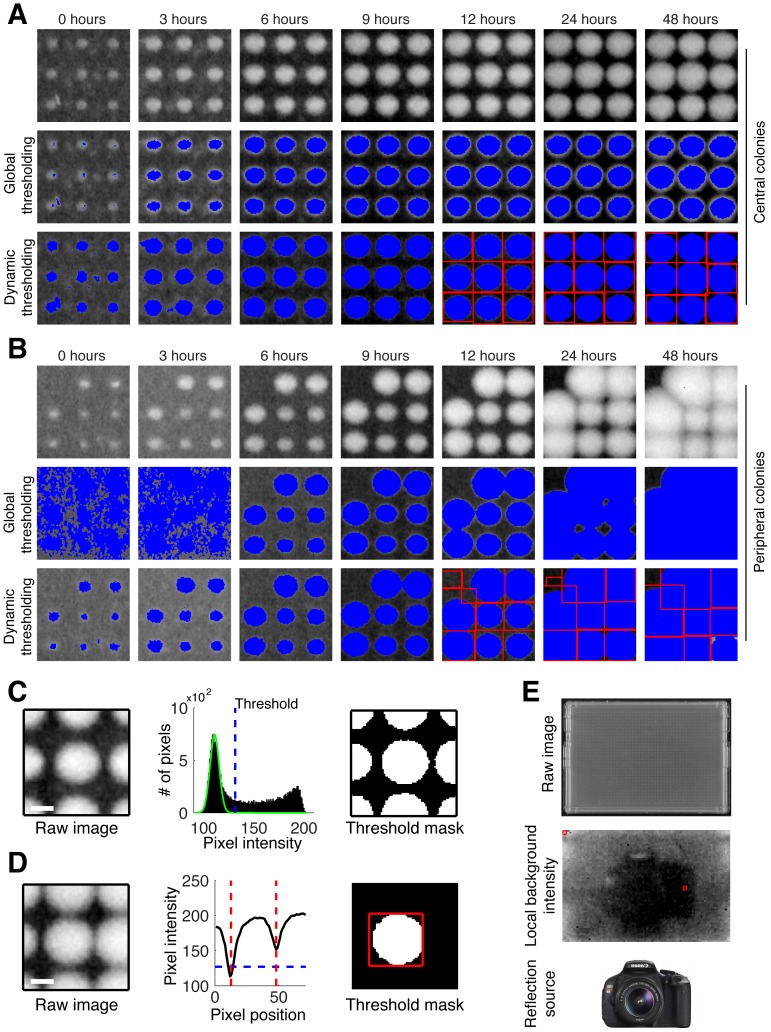
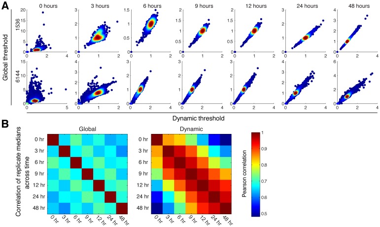
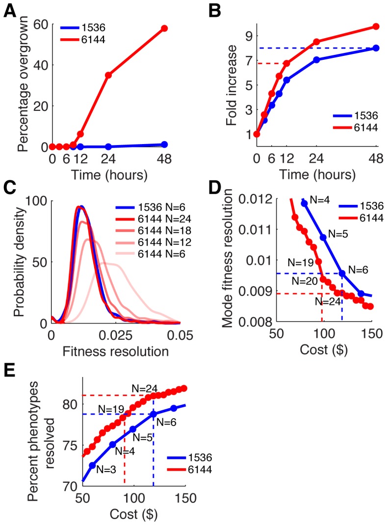
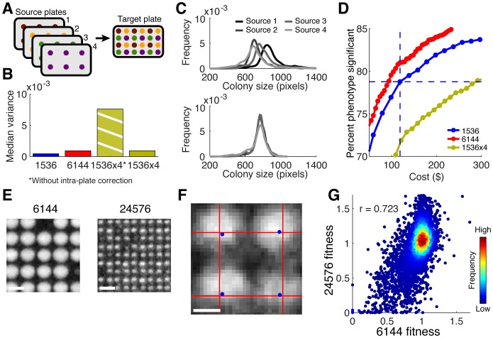
High-throughput genetic screens in model microbial organisms are a primary means of interrogating biological systems. In numerous cases, such screens have identified the genes that underlie a particular phenotype or a set of gene-gene, gene-environment or protein-protein interactions, which are then used to construct highly informative network maps for biological research. However, the potential test space of genes, proteins, or interactions is typically much larger than current screening systems can address. To push the limits of screening technology, we developed an ultra-high-density, 6144-colony arraying system and analysis toolbox. Using budding yeast as a benchmark, we find that these tools boost genetic screening throughput 4-fold and yield significant cost and time reductions at quality levels equal to or better than current methods. Thus, the new ultra-high-density screening tools enable researchers to significantly increase the size and scope of their genetic screens.

Figure 1. Experimental design and correlations between different colony densities.

(A) Diagram indicating the overlap in yeast strains used in the various-colony formats – mutants in lower density plates are always included in higher-density plates. (B) Snapshots of 384-, 1536-, and 6144-colony plates (top row, scale bar 1 mm) and mosaic view of identical mutant colonies assembled from 1536- or 6144-colony plates (zoomed) and compared to the 384-colony plate growth (bottom row). (C) To compare data quality between formats, we correlated replicates of the different formats internally or across (same format median of N = 9 replicates each; across format median of N = 18 replicates each).

Figure 2. Colony growth kinetics and colony grid alignment.

(A) Diagram of rows of larger and smaller colonies, each angled at 0.5 degrees relative to the reference (horizontal bars). Small errors in image rotation in the 6144-colony plates can lead to substantial colony identification errors. (B) Time-lapse imaging of the current 1536-density (above) and the new super-high-density format (below) reveals optimal imaging time points of 24–48 hrs for the 1536 and 12–24 hrs for the 6144 format (identical scale for all images). (C) Geometric solution for the image rotation problem. Given that the corners of the plate touch the edges of the cropped image, the width and height of the image can each be decomposed into the sum of two smaller values. These four values (X₁, X₂, Y₁, Y₂) are all trigonometric functions of θ, the angle of orientation of the grid, and the width and height of the plate. These functional relationships comprise a non-linear system of equations with a closed-form solution, which we solved for θ. (D) Snapshots of colonies growing in the middle and on the edge of 6144-colony plates; blue dots indicate the positions of the grid before (upper row) and after (lower row) the grid-adjustment step (scale bars 1 mm).

Figure 3. Comparison of global and dynamic intensity threshold algorithms.

(A, B) Snapshots of colonies in the plate center and periphery, respectively, 0, 3, 6, 9, 12, 24, and 48 hours; blue pixels in the middle and bottom rows of each panel indicate the pixels called by the respective algorithm as foreground (i.e. colony as opposed to background); red lines indicate predicted colony boundaries. The global intensity used in (A) was computed on the peripheral window, while the global intensity used in (B) was computed on the central window, highlighting the problems of global tresholding. (C) Gray-scale snapshots of a single colony at 12 hours (left, scale bar 500 µm); histograms showing the distribution of pixel intensities for the snapshot, the green curve represents the normal distribution fit to the leftmost peak (indicating the distribution of background pixel intensities), blue dotted lines indicate the threshold used to distinguish colony from background (middle); binary output (right, threshold applied) (D) Gray scale snapshot centered on an overgrown colony (left, scale bar 500 µm); line plot of median pixel intensity across the center of the snapshot (middle, blue line indicates local intensity threshold, red line indicates the colony boundary); binary image with intensity threshold and bounding box applied (right). (E) Local dynamic background estimation is very sensitive and allows for accurate colony-size estimations across a large background intensity range. Original photo of a 0-hour 6144 plate (top); grey scale heat map of the estimated background intensity for each grid position in the 0-hour image (middle; red boxes indicate the positions of the central and peripheral snapshots shown in [A,B]); the reflection of the camera used (bottom) is clearly captured by the background intensity estimation algorithm, demonstrating its sensitivity.

Figure 4. Effect of global versus dynamic background.

(A) Comparison of globally or locally/dynamically tresholded colony sizes. While good correlation is achievable between 6 and 24 hrs, poor correlation is observed at the extreme ends of the experiment. (B) In general, using dynamic local thresholding (right) achieves much better data correlation across time-points than global thresholding (left).

Figure 5. Ultra-high-density format data quality and cost efficiency.

(A) Percentage of colonies overgrown. (B) Growth curves based on median colony area fold-increase since pinning (dashed lines indicate fold increase at 12 hrs [6144] or 48 hrs [1536], N = 18 for each colony density). (C) Distribution of fitness resolutions for 1536 and 6144 format (N =  replicate numbers). (D) Mode fitness resolutions for a given cost/replicate level (dashed lines indicate equal cost/quality levels, N =  replicate numbers). (E) Percentage of single mutants that can be resolved (dashed lines indicate equal cost/quality levels, N =  replicate numbers).

Figure 6. Up-scaling and hyper-density.

(A) Schematic of the effects of up-scaling: the combination of different lower-density source plates into one higher-density target plate. (B) Comparison of variance in plates pinned with dedicated density-pads (1536, 6144) and plates using up-scaling with or without intra-plate source correction. (C) Colony size distributions obtained by the analysis pipeline without (top) and with (bottom) the intra-plate source correction. (D) Comparison of the percentage of single mutants that can be identified with a significant fitness phenotype at a given cost/replicate level (--- indicate N = 6 at 1536 density). (E) Snapshots of 6144- and 24,576 hyper-density colonies at equal scale (scale bar 1 mm). (F) Zoomed image showing jitter effect on colony placement; red grid represents perfect alignment, blue dots denote actual pin position (scale bar 100 µm). (G) Correlation of fitness measurements obtained with ultra-high- and hyper-density plates.

References

1. Uetz P, Giot L, Cagney G, Mansfield TA, Judson RS, et al. (2000) A comprehensive analysis of protein-protein interactions in Saccharomyces cerevisiae. Nature 403: 623–627 10.1038/35001009 - DOI - PubMed
1. Ito T, Chiba T, Ozawa R, Yoshida M, Hattori M, et al. (2001) A comprehensive two-hybrid analysis to explore the yeast protein interactome. Proc Natl Acad Sci USA 98: 4569–4574 10.1073/pnas.061034498 - DOI - PMC - PubMed
1. Roguev A, Bandyopadhyay S, Zofall M, Zhang K, Fischer T, et al. (2008) Conservation and rewiring of functional modules revealed by an epistasis map in fission yeast. Science 322: 405–410 10.1126/science.1162609 - DOI - PMC - PubMed
1. Costanzo M, Baryshnikova A, Bellay J, Kim Y, Spear ED, et al. (2010) The genetic landscape of a cell. Science 327: 425–431 10.1126/science.1180823 - DOI - PMC - PubMed
1. Bandyopadhyay S, Mehta M, Kuo D, Sung M-K, Chuang R, et al. (2010) Rewiring of genetic networks in response to DNA damage. Science 330: 1385–1389 10.1126/science.1195618 - DOI - PMC - PubMed
Publication types