Comparison of classifiers for decoding sensory and cognitive information from prefrontal neuronal populations

Abstract

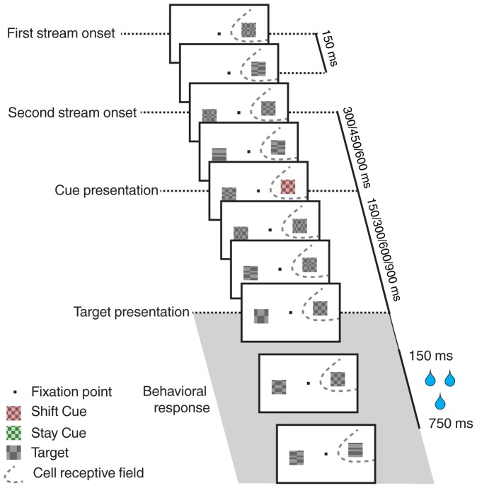
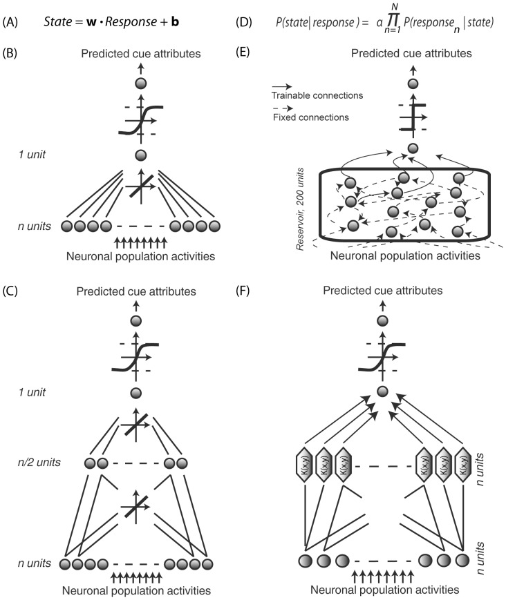
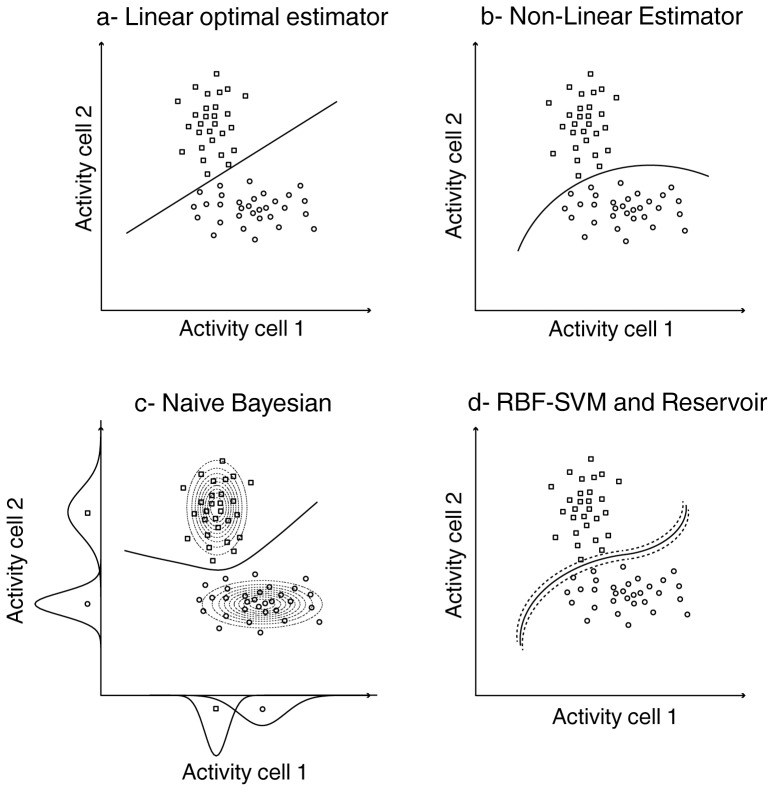
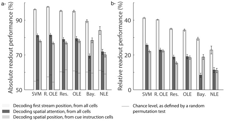
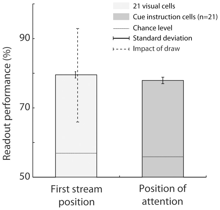
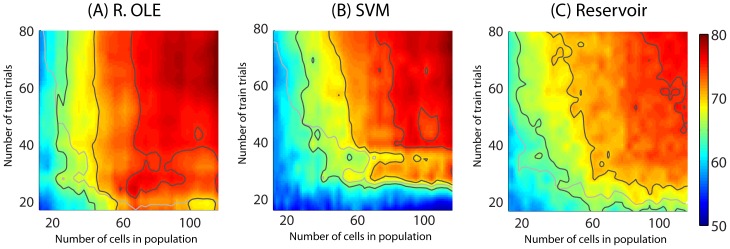
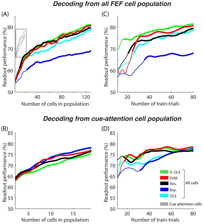
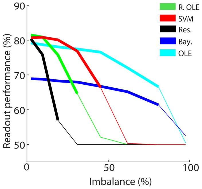
Decoding neuronal information is important in neuroscience, both as a basic means to understand how neuronal activity is related to cerebral function and as a processing stage in driving neuroprosthetic effectors. Here, we compare the readout performance of six commonly used classifiers at decoding two different variables encoded by the spiking activity of the non-human primate frontal eye fields (FEF): the spatial position of a visual cue, and the instructed orientation of the animal's attention. While the first variable is exogenously driven by the environment, the second variable corresponds to the interpretation of the instruction conveyed by the cue; it is endogenously driven and corresponds to the output of internal cognitive operations performed on the visual attributes of the cue. These two variables were decoded using either a regularized optimal linear estimator in its explicit formulation, an optimal linear artificial neural network estimator, a non-linear artificial neural network estimator, a non-linear naïve Bayesian estimator, a non-linear Reservoir recurrent network classifier or a non-linear Support Vector Machine classifier. Our results suggest that endogenous information such as the orientation of attention can be decoded from the FEF with the same accuracy as exogenous visual information. All classifiers did not behave equally in the face of population size and heterogeneity, the available training and testing trials, the subject's behavior and the temporal structure of the variable of interest. In most situations, the regularized optimal linear estimator and the non-linear Support Vector Machine classifiers outperformed the other tested decoders.

Figure 1. Task description.

The experimental procedure is a cued-target detection based on a dual rapid serial visual presentation (RSVP) paradigm. The monkey is required to maintain its gaze on the central fixation point all throughout the trial. A first stream of stimuli, that is a succession of visual stimuli every 150 ms, is presented either within (as here) or opposite the fixation point from the cell's receptive field. Three hundred milliseconds later, a second stream appears opposite the first stream from the fixation point. Three hundred, 450 or 600 ms (here, 300 ms) following the second stream onset, a cue is presented within the first stream. This cue can be a green stay cue indicating to the monkey that the target has a high probability to appear within this very same stream or a red shift cue (as here), indicating that the target has a high probability to appear within the opposite stream. On 80% of the trials, the target is presented 150, 300, 600 or 900 ms from cue onset. On 80% of these target trials (64% of all trials), the target location is correctly predicted by the cue (valid target, as here). On 20% of these target trials (16% of all trials), the target location is incorrectly predicted by the cue (invalid target). On the remaining 20% of trials, no target is presented (catch trials), so as to discourage false alarms. The target is composed of just one horizontal and one vertical spatial cycle, while distractor items are composed of up to 6 horizontal and vertical spatial cycles. The monkey gets rewarded for responding by a bar release, between 150 and 750 ms following target presentation, and for holding on to the bar when no target is presented.

Figure 2. Decoders.

(A) Regularized OLE, the training step is a simple regularized linear regression. (B) Optimal Linear Estimator (ANN OLE), implemented as a one-layer feedforward artificial neural network. The input layer has one unit per FEF cell and receives instantaneous population neuronal activities. The output layer contains 1 unit. Training involves optimizing the weights using a Levenberg-Marquardt backpropagation algorithm and a hyperbolic tangent transfer function. (C) Non-Linear Estimator (ANN NLE), implemented as a 2-layer feedforward artificial neural network. The network architecture only differs from the OLE by an additional hidden layer with n/2 units, n being equal to the number input units. (D) Bayesian decoder, applying Bayes' theorem to calculate the posterior probability that state i is being experienced given the observation of response r. (E) Reservoir decoding. The decoder has one input unit per FEF cell and one output unit. Fixed connections are indicated by dotted arrows and dynamical connections are indicated by full arrows. The reservoir contains 200 units. The recurrent connections between them are defined by the training inputs. A simple linear readout is then trained to map the reservoir state onto the desired output. (F) Support Vector Machine (SVM), the LIBSVM library (Chih-Chung Chang and Chih-Jen Lin, 2011) was used (Gaussian radial basis function kernel so as to map the training data into a higher dimensional feature space). The transformed data is then classified with a linear regressor and training is performed with a 5-fold cross-validation. For all decoders, the sign of the output corresponds to the two possible states of the variable being decoded.

Figure 3. Decision boundaries for the different classifiers.

Each plot represents the activity of a hypothetical cell 1 as a function of the activity of hypothetical cell 2, on successive trials, in response to a stimulus 1 (circles) or 2 (squares). a) Optimal linear estimator; b) non-linear estimator; c) naive Bayesian. The dotted ellipsoids (Bayesian) correspond to the probability-density fitted Gaussian distributions of the cells' activities for each stimulus; d) SVM with Gaussian kernel (RBF) and Reservoir. In the case of SVM, the dotted line corresponds to the margin around the decision boundary.

Figure 4. Comparison of mean performance at reading out first stream position and spatial attention across classifiers.

A) Absolute readout performance. The dashed lines indicate the chance level for each condition, as estimated by a random permutation test (p<0.05). B) Readout performance, relative to chance level. The flow position is decoded using all cells in the population (light gray). Spatial attention is decoded using all cells in population (dark gray) or using only cells with significant individual attention-related responses (intermediate gray). The mean readout performance and the associated standard error around this mean are calculated over 20 decoding runs. SVM  =  support vector machine, Res.  =  reservoir, R. OLE  =  regularized OLE, Bay.  =  Bayesian, NLE  =  ANN non-linear estimator, OLE  =  ANN optimal linear estimator.

Figure 5. Comparison of decoding flow onset (light gray) with 21 visual cells versus decoding spatial position of attention (dark gray) with the 21 cells with significant individual attention-related responses.

The mean read-out performance across 20 runs is showed with standard deviation around this mean. The dotted line corresponds the maximum- and minimum performance across 20 draws of 21 visual cells out of 111. The SVM classifier was used. The mean readout performance and the associated standard error around this mean are calculated over 20 decoding runs. Chance level is defined using a random permutation procedure (p<0.05).

Figure 6. Decoding of spatial attention from the whole FEF population activities as a combined function of number of trials and cells with (A) Regularized OLE, (B) SVM and (C) Reservoir decoders.

The black contour lines correspond, from yellow to dark red regions, to 65, 70 and 75% of readout performance. The gray contour lines corresponds to chance level as calculated, at each point, by a random permutation test (p<0.05). Smoothing with Gaussian kernel of 7. The readout performance is an average readout performance on 10 decoding runs. The maximum possible number of training trials is 84 trials. The y-axes are truncated at 80 trials.

Figure 7. Decoding spatial attention (A–B) as a function of cell population size and (C–D) number of trials available for training.

In (A) and (C), decoding is performed on the whole FEF cell population while in (B) and (D), decoding is performed only on the attention-related cells -presented also in gray in (A). The mean readout performance is calculated over 20 decoding runs. Thick lines indicated values that are significantly above chance as calculated using a random permutation test (p<0.05). SVM  =  support vector machine, Res  =  reservoir, Ex. OLE  =  explicit OLE, Bay.  =  Bayesian, NLE  =  ANN non-linear estimator, OLE  =  ANN optimal linear estimator.

Figure 8. Impact of imbalance in the training set.

The y-axis represents the difference between the readout performance of a balanced data set (same number of trials for each condition) and that of an unbalanced data set (more trials in condition 1 than in condition 2). The x-axis represents the degree of imbalance in training trial number between the two conditions. The mean readout performance and the associated standard error around this mean are calculated on 20 decoding runs. Thick lines indicated values that are significantly above chance as calculated using a random permutation test (p<0.05). SVM  =  support vector machine, Res  =  reservoir, R. OLE  =  regularized OLE, Bay.  =  Bayesian, NLE  =  ANN non-linear estimator, OLE  =  ANN optimal linear estimator.

Figure 9. Impact of memory on Reservoir decoding performance on reading out the spatial position of attention.

The light gray curve and bars corresponds to a reservoir training on a window of 75(as in all previous figures). The dark gray curve and bars corresponds to a reservoir training a larger time window (from cue onset at 0 ms to 700 ms post-cue). Decoding is performed on all FEF cell population activities. The bars show the mean readout performance and the associated standard error around this mean obtained by testing activities in a time window of 100 ms around the time reference point for training (245 ms after cue onset, N = 20 decoding runs). The curves show the mean readout performance and the associated standard error around this mean for each time point. Thick lines indicated values that are significantly above chance as calculated using a random permutation test (p<0.05).

References

1. Ben Hamed S, Page W, Duffy C, Pouget A (2003) MSTd neuronal basis functions for the population encoding of heading direction. J Neurophysiol 90: 549–558. - PubMed
1. Ben Hamed S, Schieber MH, Pouget A (2007) Decoding M1 neurons during multiple finger movements. J Neurophysiol 98: 327–333. - PubMed
1. Musallam S, Corneil BD, Greger B, Scherberger H, Andersen RA (2004) Cognitive control signals for neural prosthetics. Science 305: 258–262. - PubMed
1. Armstrong KM, Chang MH, Moore T (2009) Selection and maintenance of spatial information by frontal eye field neurons. J Neurosci 29: 15621–15629. - PMC - PubMed
1. Gu Y, Fetsch CR, Adeyemo B, Deangelis GC, Angelaki DE (2010) Decoding of MSTd population activity accounts for variations in the precision of heading perception. Neuron 66: 596–609. - PMC - PubMed
Publication types
LinkOut - more resources