Saliency mapping in the optic tectum and its relationship to habituation

Abstract

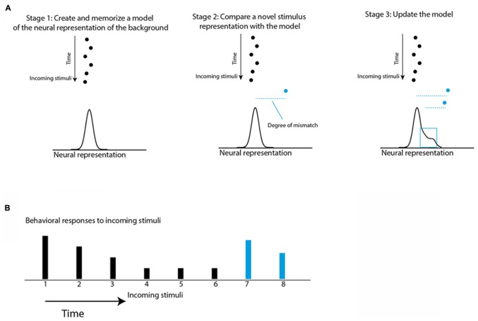
Habituation of the orienting response has long served as a model system for studying fundamental psychological phenomena such as learning, attention, decisions, and surprise. In this article, we review an emerging hypothesis that the evolutionary role of the superior colliculus (SC) in mammals or its homolog in birds, the optic tectum (OT), is to select the most salient target and send this information to the appropriate brain regions to control the body and brain orienting responses. Recent studies have begun to reveal mechanisms of how saliency is computed in the OT/SC, demonstrating a striking similarity between mammals and birds. The saliency of a target can be determined by how different it is from the surrounding objects, by how different it is from its history (that is habituation) and by how relevant it is for the task at hand. Here, we will first review evidence, mostly from primates and barn owls, that all three types of saliency computations are linked in the OT/SC. We will then focus more on neural adaptation in the OT and its possible link to temporal saliency and habituation.

Keywords: barn owl; habituation; optic tectum; orienting response; saliency map; spatial attention; superior colliculus.

FIGURE 1

Schematic illustration of a conceptual model of habituation and saliency mapping. (A) The black dots represent a stream of stimuli coming one after the other in time. The horizontal positions represent points on the internal neural representation axis. The statistics of the incoming stimuli are learned and memorized in Stage 1 to create an expectation model that is the expected probability of the internal representation of the next stimulus. The expectation model is illustrated by a normal curve. The blue dot is a new incoming stimulus. In Stage 2, the expectation violation of the new stimulus is measured based on the degree of mismatch between the internal representation of the new stimulus and the memorized model (dashed blue line). Then, in Stage 3 the representation of the new stimulus is incorporated into the model to affect the degree of mismatch of further incoming stimuli. (B) The height of the bars represents the predicted behavioral responses to the incoming stimuli (dots in A) based on the assumption that each response is proportional to the degree of mismatch.

FIGURE 2

Illustration showing a selected part of the barn owl’s auditory pathway with the OT as a hub. Gray boxes indicate structures suggested to be related to gaze and attention control. The red outline indicates structures where SSA was reported; the blue outline indicates areas where long-term adaptation was reported (habituation-like responses); the yellow outline indicates structures where multisensory (visual/auditory) neurons were reported. Double-headed arrows indicate reciprocal connections. Abbreviations of names of structures appear within each box. The abbreviations of names of the equivalent mammalian structures are in parentheses: E, entopallium; AGF, arcopallium gaze fields; FEF, frontal eye fields; nRt, nucleus rotundus; OTs, superficial layers of the OT (layers 1–10); OTi/s, intermediate and deep layers of the OT (layers 11–15); IC, inferior colliculus; Ipc, nucleus isthmi pars parvocellularis; Imc, nucleus isthmi pars magnocellularis; nOv, nucleus ovoidalis; MGN, medial geniculate body; A1, auditory cortex 1.

FIGURE 3

Pupil dilation responses (PDRs) and microstimulation in the OT. (A) The left image shows a zoomed image of a barn owl’s right eye. The image is a video frame taken from an infra-red sensitive video sequence showing the infra-red light reflected from the retina. The arrow points to the edge of the pecten, a retinal landmark absorbing light. The image on the left shows a similar video frame after processing and fitting the pupil edge with an ellipse. The red circle designates the fitted pupil edge. The cross designates the center of the circle and the blue line shows the horizontal edge of the pecten. The diameter of the circle and the average horizontal position of the pecten edge were used to measure pupil dilations and eye movements. (B) The graph shows PDRs to three consecutive auditory stimuli given every 12 s. The solid line designates the response to the first stimulus, the dashed line the response to the second stimulus and the dotted line the response to the third stimulus. The base line of all response profiles was reduced to zero level. The horizontal bar indicates the duration of the acoustic stimulus and the vertical line the onset of stimulation. (C) Results of coupling acoustic and tectal electrical stimulation. The inset shows the time course of the stimulation protocol. Auditory stimuli were repeated every 12 s (gray bars). Occasionally, with a probability of 20%, a brief low-level microstimulation was injected shortly before the auditory stimulus (blue bars). The gray curve shows the population average PDR to the repeated auditory stimulus. The red curve shows the population average PDR to the auditory stimuli that followed a microstimulation. Note the release from habituation. (D) The inset shows the time course of the experiment. The gray vertical bars indicate auditory stimuli and the blue vertical bars electrical stimulations. Auditory stimuli were repeated every 10 s alternating between two positions: one matching the electrical stimulation site in the tectal map and the other not matching the electrical stimulation site. The gray curves show the population PDRs to the two auditory stimuli. The blue curve shows the population PDR to the non-matched auditory stimuli that were coupled with the microstimulation, and the red curve the population PDR to the matched auditory stimuli coupled with the microstimulation. Microstimulation at the site corresponding with the acoustic stimulus induces a stronger release from habituation. Modified from Netser et al. (2010).

FIGURE 4

Stimulus protocols used to differentiate stimulus-specific adaptation (SSA) from non-specific adaptation. (A) The priming protocol. In the priming protocol a tuning curve is generated by presenting sequences of stimuli varying randomly over a range of stimuli (f1–fn). This is repeated in two conditions: in one, the stimuli for generating the tuning curve are spaced with a fixed time interval of no stimulation (the control); in the other, in between stimuli, a standard stimulus (fs) is presented several times. In non-specific adaptation (left graph), the tuning curve in the primed condition (gray curve) is expected to be attenuated evenly relative to the control. In SSA, the adaptation is expected to occur stronger near the fs stimulus, resulting in a dip in the tuning curve. (B) The oddball protocol. In the oddball protocol, two different stimuli are chosen (f1 and f2) so that both are within the response range of the neuron, giving rise to about the same response. One stimulus is chosen as the standard, being presented repeatedly for a long period. Within this sequence, the second stimulus, called the deviant, is embedded with a relatively low probability. Later, a second block is presented in which the roles are changed: the stimulus that was standard is now deviant, and vice versa. At the end of the experiments, the average responses to the standards are compared with the corresponding responses to the deviants. In non-specific adaptation, we expect no significance differences (left histogram). In SSA, we expect the responses to the deviant to appear consistently above the responses to standards (right histogram). (C) The constant order protocol. Two stimuli are presented in a long sequence, starting with several repetitions of f1 then switching to several repetitions of f2, and so on, alternating between the two stimuli. In non-specific adaptation, we expect that the response to the first stimulus in each sub-sequence will be adapted and therefore not larger than the response to the same stimulus when it is last in the sequence. In SSA, we expect a stronger response every time the sequence is switched from one stimulus to the other (right histogram in C). Modified from Gutfreund (2012).

FIGURE 5

(A) The histogram shows the average response of a population of neurons in the OT to a long sequence of stimuli (200 stimuli). The duration of each stimulus was 200 ms and the ISI was 1 s. The sequence alternated between two ITD values; every 10 repetitions the ITD of the sound was switched to the other value (protocol is illustrated in the inset at the bottom of the figure). The graph on the right shows the post-stimulus time histogram (PSTH) of one stimulus when it was first in its sub-sequence (deviant, light red curve) compared to the PSTH for the same stimulus when it was last in its sub-sequence (standard, black curve). (B) Same as A, but in this case, the two stimuli were narrowband stimuli (width of 1 kHz) differing in their central frequency. (C) Same as A and B, but in this case, the two stimuli differed in intensity. One stimulus (dark blue bars) was softer compared to the other (light red bars). The average response to deviant stimulus was greater in all cases. Modified with permission from Reches and Gutfreund (2008). (D,E) Two examples of tectal recordings showing bimodal enhancement. The raster plots show results of unit responses to a sequence of five repetitions of a stimulus with an ISI of 800 ms. The time course of stimulation is designated by the horizontal black bars. Stimuli were either five visual stimuli, five auditory stimuli, or five congruent bimodal stimuli (visual and auditory stimuli appearing together from the same location). The solid vertical line designates the onset of the first stimulus in the sequence. The dashed vertical lines designate the onset of subsequent stimuli. In both examples (D,E), stronger responses to bimodal stimuli can be seen in the response to the first stimulus in the sequence compared to the unimodal responses. This bimodal enhancement is missing in the responses to the subsequent stimuli. Modified from Zahar et al. (2009).

References

1. Adolphs R. (1993). Bilateral inhibition generates neuronal responses tuned to interaural level differences in the auditory brainstem of the barn owl. J. Neurosci. 13 3647-3668 - PMC - PubMed
1. Albeck Y., Konishi M. (1995). Responses of neurons in the auditory pathway of the barn owl to partially correlated binaural signals. J. Neurophysiol. 74 1689–1700 - PubMed
1. Anderson B. A. (2013). A value-driven mechanism of attentional selection. J. Vis. 13 7 10.1167/13.3.7 - DOI - PMC - PubMed
1. Anderson L. A., Christianson G. B., Linden J. F. (2009). Stimulus-specific adaptation occurs in the auditory thalamus. J. Neurosci. 29 7359–7363 10.1523/JNEUROSCI.0793-09.2009 - DOI - PMC - PubMed
1. Antunes F. M., Nelken I., Covey E., Malmierca M. S. (2010). Stimulus-specific adaptation in the auditory thalamus of the anesthetized rat. PLoS ONE 5:e14071 10.1371/journal.pone.0014071 - DOI - PMC - PubMed
LinkOut - more resources