. 2014 Mar;17(3):440-8.
doi: 10.1038/nn.3643. Epub 2014 Feb 2.

Cortical activity in the null space: permitting preparation without movement

Affiliations

Cortical activity in the null space: permitting preparation without movement

Matthew T Kaufman et al. Nat Neurosci. 2014 Mar.

Abstract

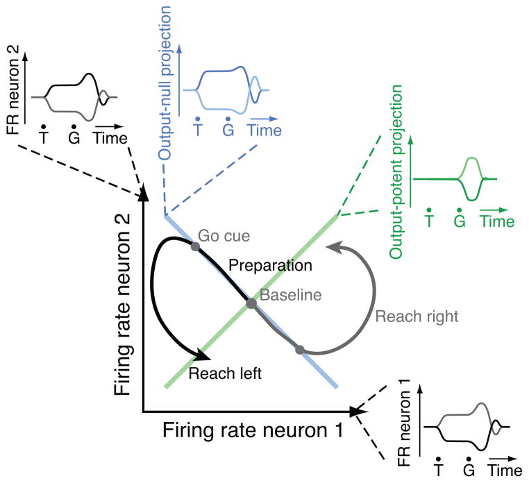
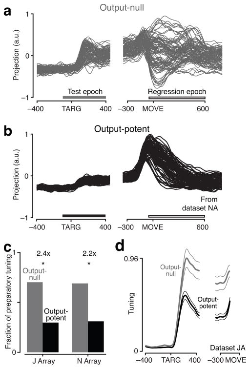
Neural circuits must perform computations and then selectively output the results to other circuits. Yet synapses do not change radically at millisecond timescales. A key question then is: how is communication between neural circuits controlled? In motor control, brain areas directly involved in driving movement are active well before movement begins. Muscle activity is some readout of neural activity, yet it remains largely unchanged during preparation. Here we find that during preparation, while the monkey holds still, changes in motor cortical activity cancel out at the level of these population readouts. Motor cortex can thereby prepare the movement without prematurely causing it. Further, we found evidence that this mechanism also operates in dorsal premotor cortex, largely accounting for how preparatory activity is attenuated in primary motor cortex. Selective use of 'output-null' vs. 'output-potent' patterns of activity may thus help control communication to the muscles and between these brain areas.


Figures

Figure 1
Figure 1
Illustration of task and of typical data. a. Layout of maze task. One typical trial shown. The same mazes were repeated many times; each maze is hereafter called a ‘condition.’ b. Top, task timeline. The monkey initially touched a central spot, then a target and (typically) barriers appeared. On some trials, two inaccessible distractor ‘targets’ also appeared. After the Go cue, the monkey made a curved reach (which left a white trail on the screen) around the barriers to touch the accessible target. Middle, trial-averaged deltoid EMG. Bottom, firing rate of one PMd neuron. Times are target onset, go cue, and movement onset. Flanking traces show s.e.m. Maze ID100, neuron J-PM48, EMG recording J-PD10.
Figure 2
Figure 2
Simplified output-null model. For illustration, assume a muscle receives input from two neurons and produces a response that is the linear sum of the inputs. If the sum is constant (“Output-null dimension”), the muscle cannot distinguish between input 1 being high and 2 low, or vice versa. When the sum changes (“Output-potent dimension”), muscle output will change. If preparatory neural activity changes only within the output-null dimension (two different reaches illustrated), then the muscle’s activity remains constant; when neural activity changes in the output-potent dimension also, movement ensues. Insets: PSTHs for the neurons, and PSTH-like views of output-potent and output-null dimensions. T, target onset, G, go cue.
Figure 3
Figure 3
Examples suggesting potential output-null structure. a. When the weighted activity of the left neuron is added to the activity of the center neuron, the result (right) has less preparatory activity than either input. This pair thus illustrate the output-null idea, though with more neurons a more complete cancellation occurs. Constant c was set to 0.37. Conditions colored based on preparatory activity of left neuron. b. Example readouts of real data. Each panel shows a linear, two-dimensional readout of real data, exhibiting the predicted structure (compare with Fig. 2). Each trace corresponds to a single, trial-averaged condition. Preparatory activity shown in blue, movement activity shown in green, and state at Go cue shown as grey circles. Red ellipse shows 2 s.d. of the preparatory activity. As in the model, preparatory activity for different conditions is mostly spread out in one dimension, while movement-epoch activity travels through both dimensions. Dimensions found using jPCA.
Figure 4
Figure 4
Output-null results for cortex to muscles. a. Neural activity in one output-null dimension for one dataset (JA-2D1). All activity is trial-averaged, and each trace represents the response for a different condition. b. Neural data in one output-potent dimension. Dimensions were identified relative to EMG activity. This pair of example dimensions has a tuning ratio of 9.2. Bars indicate “test epoch” (−100 to +400 ms from target onset), where the tuning ratio was computed, and “regression epoch” (−50 to +600 ms from movement onset), where dimensions were identified. c. Fraction of preparatory tuning (across conditions and times) in output-null (gray) and output-potent (black) dimensions for each dataset. Tuning ratios indicated above bars; all values were significantly greater than unity. d. Tuning at each time-point, in the output-null and output-potent dimensions. Flanking traces indicate s.e.m. computed via resampling of conditions.
Figure 5
Figure 5
Testing analysis method on simulated data. Simulations produced artificial neural and EMG “recordings” with the desired strength of output-null structure (Methods). Our analysis was run on this artificial data to quantify accuracy. a. Example real neural recording. Each trace shows trial-averaged response for one condition. Conditions color-coded according to preparatory activity level. b. Example simulated neuron. Qualitatively, it exhibits similar response complexity to real neuron. c. Example real EMG recording. d. Example simulated EMG recording. Qualitatively, it exhibits similar response complexity to real muscle. e. Analysis of data produced without distorting nonlinearities. Dot indicates median measured effect size for set of 50 simulations. Error bars encompass 68% of simulations (equivalent to 1 s.d.). Grey line shows unity. f. Analysis of data distorted with floor effects and saturating nonlinearities. g. Analysis of same data as in f, but underlying dimensionality was “underestimated” during analysis: two output-null and two output-potent instead of three and three. h. Same as g, but dimensionality overestimated as four output-null and four output-potent. In essentially all cases, adding nonlinearities to the data or misestimating dimensionality (including unequal numbers of output-null and output-potent dimensions; Supplementary Fig. 3) resulted in underestimates, not overestimates, of true effect size. Our results are thus likely conservative.
Figure 6
Figure 6
Output-null results for PMd to M1. Format as in Figure 4. a. Neural activity in one PMd output-null dimension for one dataset (NA-D4). b. Neural activity in one PMd output-potent dimension. Dimensions were identified relative to M1 activity. This example pair of dimensions has a tuning ratio of 3.8. c. Fraction of preparatory and baseline tuning (across conditions and times) in output-null (gray) and output-potent (black) dimensions for each dataset. Both ratios were significantly greater than unity. d. Tuning at each time-point, in the output-null and output-potent dimensions. Flanking traces indicate s.e.m. computed via resampling of conditions.
Figure 7
Figure 7
Controls for output-null analysis. a. Results of output-null analysis, with M1 as ‘source’ and PMd as ‘target’. As expected, no substantial effect was found. b. Muscle activity over time relative to key epochs. Each muscle’s activity was first normalized by its range. Heavy trace indicates mean across muscles. Width of thin traces shows mean tuning depth (assessed as standard deviation across conditions). Red bar shows epoch used to identify output-potent dimensions. Effect size computed using only preparatory data (black bar). Monkey J. c. Black bars show measured effect size for each dataset. Blue bars show effect size due to neurons with strong preparatory tuning preferentially contributing to output-null dimensions. Chance is unity. d. Neurons’ contributions to the output-null and output-potent dimensions. For each neuron, a space preference index was computed, which is +1 if the neuron contributes solely to output-potent dimensions and −1 if the neuron contributes solely to output-null dimensions. Histogram of values from the data are plotted in black (dataset J). Chance distribution is plotted in purple. Horizontal bars (above) show ±1 SD. Dots indicate means. Values for examples below indicated by green arrowheads. e. PSTH for example neuron that mainly contributed to output-null dimensions. Unit J36. f. Same as e, for neuron that contributed almost equally to output-null and output-potent dimensions. Unit J2. g. Same as e, for neuron that mainly contributed to output-potent dimensions. Unit J149.

Comment in

References

    1. Haider B, McCormick DA. Rapid neocortical dynamics: cellular and network mechanisms. Neuron. 2009;62:171–189. - PMC - PubMed
    1. Pesaran B, Nelson MJ, Andersen RA. Free choice activates a decision circuit between frontal and parietal cortex. Nature. 2008;453:406–409. - PMC - PubMed
    1. Cisek P, Puskas GA, El-Murr S. Decisions in changing conditions: the urgency-gating model. J Neurosci. 2009;29:11560–11571. - PMC - PubMed
    1. Ditterich J. Evidence for time-variant decision making. Eur J Neurosci. 2006;24:3628–3641. - PubMed
    1. Green AM, Kalaska JF. Learning to move machines with the mind. Trends Neurosci. 2011;34:61–75. - PubMed

Publication types

LinkOut - more resources