Cell lineage tracing in the developing enteric nervous system: superstars revealed by experiment and simulation

Abstract

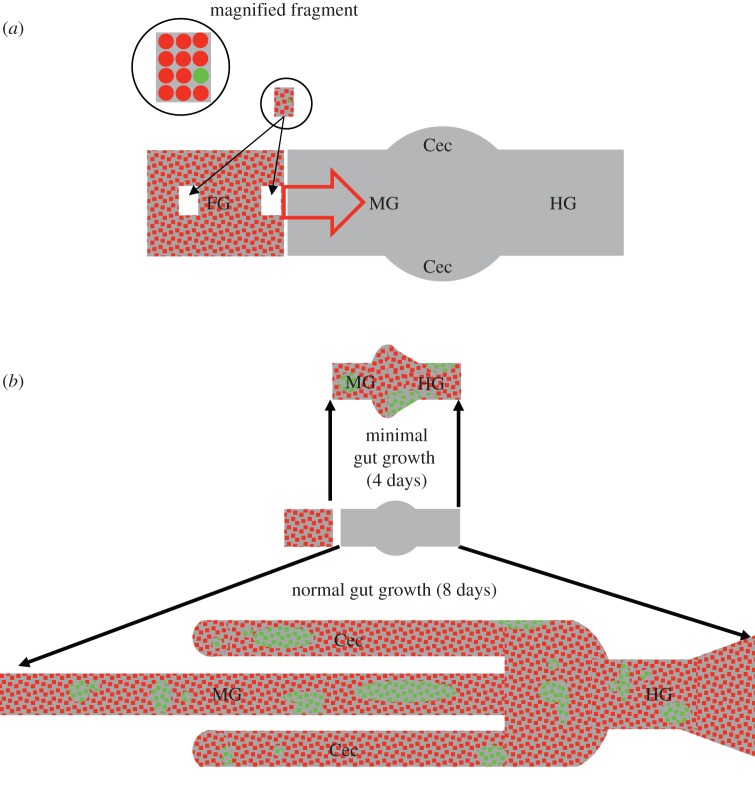
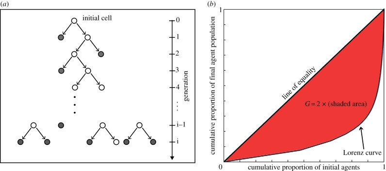
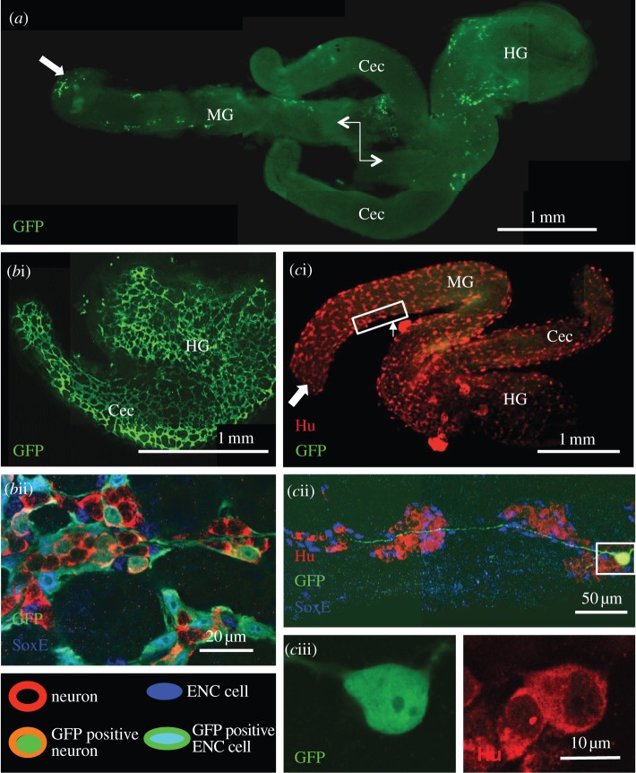
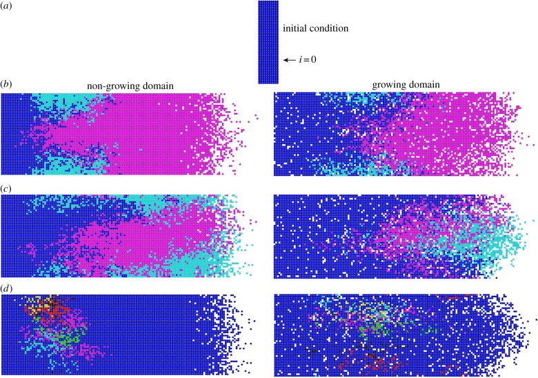
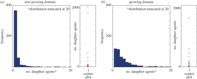
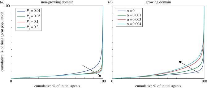
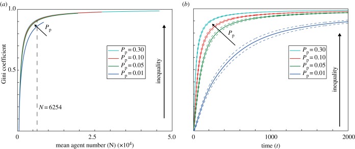
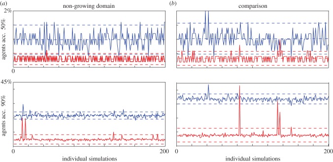
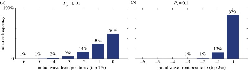
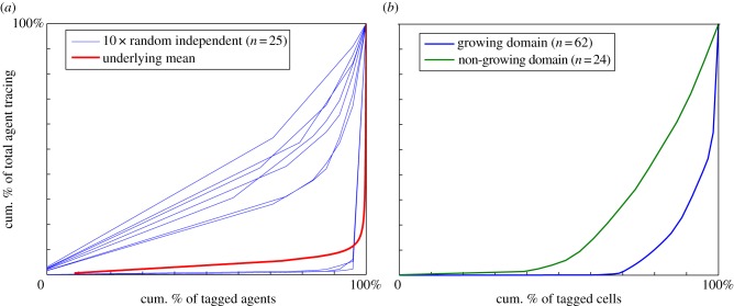
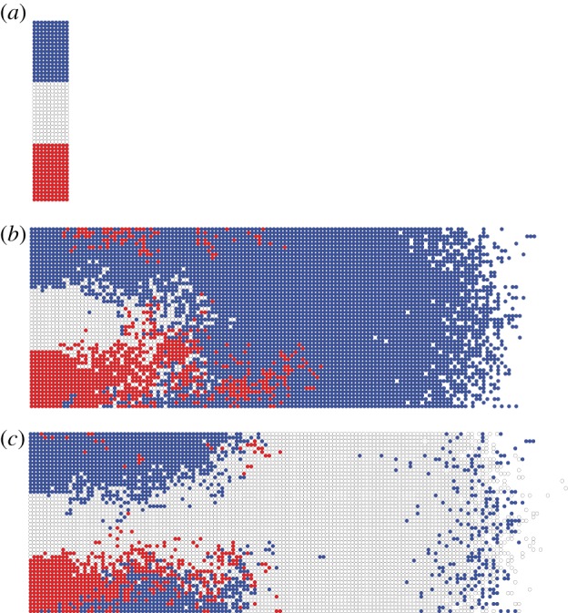
Cell lineage tracing is a powerful tool for understanding how proliferation and differentiation of individual cells contribute to population behaviour. In the developing enteric nervous system (ENS), enteric neural crest (ENC) cells move and undergo massive population expansion by cell division within self-growing mesenchymal tissue. We show that single ENC cells labelled to follow clonality in the intestine reveal extraordinary and unpredictable variation in number and position of descendant cells, even though ENS development is highly predictable at the population level. We use an agent-based model to simulate ENC colonization and obtain agent lineage tracing data, which we analyse using econometric data analysis tools. In all realizations, a small proportion of identical initial agents accounts for a substantial proportion of the total final agent population. We term these individuals superstars. Their existence is consistent across individual realizations and is robust to changes in model parameters. This inequality of outcome is amplified at elevated proliferation rate. The experiments and model suggest that stochastic competition for resources is an important concept when understanding biological processes which feature high levels of cell proliferation. The results have implications for cell-fate processes in the ENS.

Keywords: cell lineage; cell-fate decisions; enteric nervous system; invasion wave.

Figure 1.

Schematic diagram of the ENS experiments. (a) Diagram of culture system set-up. Quail E4 foregut (FG) with ENC cells (red (mid-grey) dots) is supplemented with a fragment of E3.5 FG with one GFP positive ENC cell (green (light grey) dot). This is placed either centrally or at the distal edge of the FG. This moiety is fused to an E4 post-umbilical midgut (MG) and hindgut (HG) with bilateral cecae (Cec). This gut region is uncolonized by ENC cells. Colonization then proceeds in an MG to HG wave of ENC cells (large red arrow). (b) The initial set-up is grown either for 4 days as an organ culture in vitro, where there is minimal tissue growth, or for 8 days as a CAM graft where the gut grows similarly to normal. The uncolonized MG and HG becomes occupied by ENC cells (red (mid-grey) dots) including clonal derivatives of the original GFP positive ENC cell. These GFP positive derivatives show unpredictable numbers and distributions at the end of the growth period. (Online version in colour.)

Figure 2.

Schematic lineage tracing diagram and a Lorenz curve. (a) Lineage of a single agent at time t. An empty circle represents an agent division event. Only the grey-filled circles are counted to determine the agent lineage. (b) Lorenz curve and Gini coefficient G, which is twice the shaded region. (Online version in colour.)

Figure 3.

Normal gut growth. Grafts of midgut (MG), cecae (Cec) and hindgut (HG) after 8 days growth on CAM, with descendants of a single GFP positive ENC cell shown in green. (a) Specimen in which GFP positive cells are scattered along the intestine, from the original donor position in the rostral MG, indicated by broad arrow, to the HG. (b(i)) Confocal views of a superstar specimen with huge numbers of GFP positive cells densely forming the myenteric plexus throughout the intestine. (b(ii)) At higher magnification, triple labelling shows that the ENS ganglia contain both neurons (Hu label, red) and glial/ENC cells (SoxE label, blue), with GFP positive and negative cells in both categories. (c(i)) Specimen with only one GFP positive cell. This cell occurred in the MG (thin arrow), far displaced from the original donor position (broad arrow). Note that the entire gut is colonized, shown by ENS ganglia (Hu label). (c(ii)) Enlargement of the boxed area in (c(i)) shows this GFP positive cell extended a long axon rostrally through other ENS ganglia. (c(iii)) Enlargement of the boxed area in (c(ii)) confirms that this GFP positive cell is a neuron, with strong Hu labelling (red).

Figure 4.

Spatial distribution of agent tracings for non-growing and growing (α = 0.003) domain simulations, P_p = 0.05. (a) Initial condition for all simulations. Each fully occupied column has an index i, where i = 0 corresponds to the right-most column. (b,c) Largest lineage tracing (pink), second largest lineage tracing (turquoise) and remaining agent population (blue). (b) Significant differences in the agent numbers between the two largest tracings. (c) The two largest tracings have a similar number of agent numbers. (d) The fifth to tenth largest tracings in (c). The total number of agents in (b–d) is the same. For the non-growing case this occurs at t ≈ 600, whereas for the growing case, t ≈ 400.

Figure 5.

Single realization frequency distribution and scatter plot (500 data points), P_p = 0.05. (a) Non-growing domain, α = 0. (b) Growing domain, α = 0.003. Note the distributions in the histograms are truncated. (Online version in colour.)

Figure 6.

Lorenz curves. (a) Non-growing domain, α = 0. The arrow indicates increasing proliferation probability P_p. (b) Growing domain, with P_p = 0.05. The arrow indicates increasing domain growth rate α. The curves show that a small proportion of the initial starting population is contributing to bulk of the total agent population. (Online version in colour.)

Figure 7.

Gini coefficient for non-growing domain and various proliferation rates P_p. (a) As a function of average total agent number. The vertical dashed line indicates the total agent number used in the Lorenz curves of figure 6a. (b) As a function of time (solid lines). The dashed lines indicate the 95% confidence intervals (±1.95σ). (Online version in colour.)

Figure 8.

Consistency of superstars across 200 individual realizations. Smallest % of agent tracings required to account for 50% (top panels) and 90% (bottom panels) of final agent population. The mean and 95% confidence interval (±1.95σ) are shown with dashed lines. (a) Non-growing domain for two values of the probability of proliferation P_p = 0.01 (blue upper curve) and P_p = 0.1 (red lower curve). (b) Comparison between growing (blue upper curve, α = 0.003) and non-growing domains with P_p = 0.05 (red lower curve). (Online version in colour.)

Figure 9.

Column Lorenz curves L(i)_hi for different proliferation rates P_p. The position i indicates the position relative to the wavefront, where i = 0 corresponds to the wavefront. The stacked bar chart on the right of each subfigure indicates each column’s average percentage contribution to the final population. (a–d) P_p = 0.01, 0.05, 0.1, 0.3. (Online version in colour.)

Figure 10.

Frequency distribution of the initial position i relative to the wavefront of the largest 2% of lineage tracings across 200 simulations for two values of the proliferation rate. (a) P_p = 0.01; (b) P_p = 0.1. (Online version in colour.)

Figure 11.

Comparison between simulation and experimental Lorenz curves. (a) Ten Lorenz curves (blue) from randomly sampling a single agent from n = 25 in silico non-growing experiments, P_p = 0.05 and α = 0. Lorenz curve (red thicker lower curve) from a single in silico experiment where all initial agents are tagged (indistinguishable from the one in figure 6 with same P_p and α values). (b) Lorenz curve from the experimental data (combining the wavefront and behind the wavefront data) in table 1 (no growth, blue lower curve) and table 2 (growth, green upper curve). (Online version in colour.)

Figure 12.

Two simulation results if agents have a predetermined fate before the invasion process commences (non-growing case). (a) Initial condition with three cell fates. (b,c) Two realizations with very different outcomes. Here, P_p = 0.05.

References

1. Kretzschmar K, Watt FM. 2012. Lineage tracing. Cell 148, 33–45. (10.1016/j.cell.2012.01.002) - DOI - PubMed
1. Livet J, Weissman TA, Kang H, Draft RW, Lu J, Bennis RA, Sanes JR, Lichtman JW. 2007. Transgenic strategies for combinatorial expression of fluorescent proteins in the nervous system. Nature 450, 56–62. (10.1038/nature06293) - DOI - PubMed
1. Lichtman JW, Livet J, Sanes JR. 2008. A technicolour approach to the connectome. Nat. Rev. Neurosci. 9, 417–422. (10.1038/nrn2391) - DOI - PMC - PubMed
1. Pan YA, et al. 2013. Zebra bow: multispectral cell labeling for cell tracing and lineage analysis in zebrafish. Development 140, 2835–2846. (10.1242/dev.094631) - DOI - PMC - PubMed
1. Naik SH, Perie L, Swart E, Gerlach C, van Rooij N, de Boer RJ, Schumacher TN. 2013. Diverse and heritable lineage imprinting of early haematopoietic progenitors. Nature 7444, 229–232. (10.1038/nature12013) - DOI - PubMed
Publication types
LinkOut - more resources