A map of functional synaptic connectivity in the mouse anteroventral cochlear nucleus

Abstract

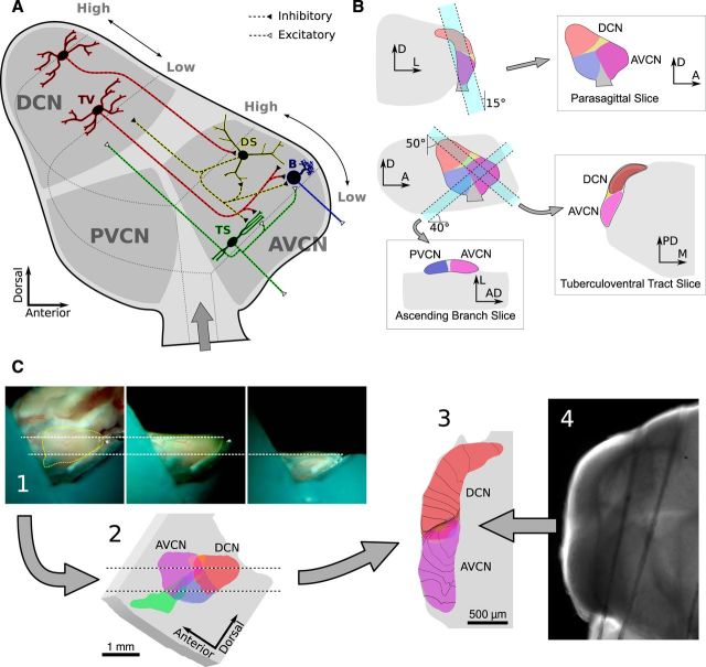
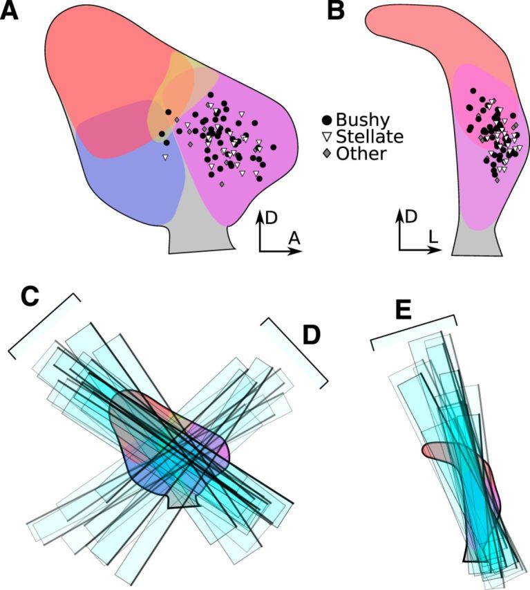
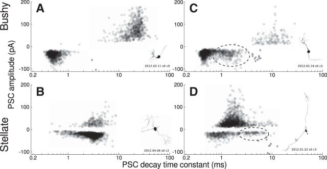
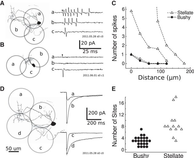
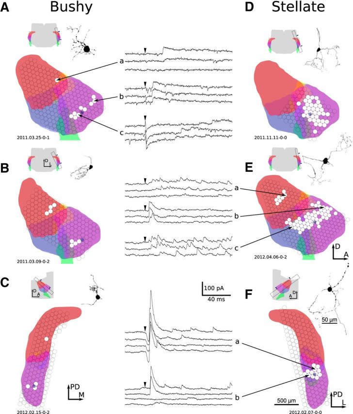
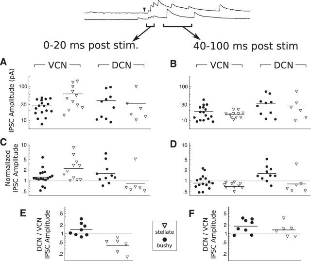
The cochlear nuclei are the first central processors of auditory information and provide inputs to all the major brainstem and midbrain auditory nuclei. Although the local circuits within the cochlear nuclei are understood at a cellular level, the spatial patterns of connectivity and the connection strengths in these circuits have been less well characterized. We have applied a novel, quantitative approach to mapping local circuits projecting to cells in the mouse anteroventral cochlear nucleus (AVCN) using laser-scanning photostimulation and glutamate uncaging. The amplitude and kinetics of individual evoked synaptic events were measured to reveal the patterns and strengths of synaptic connections. We found that the two major excitatory projection cell classes, the bushy and T-stellate cells, receive a spatially broad inhibition from D-stellate cells in the AVCN, and a spatially confined inhibition from the tuberculoventral cells of the dorsal cochlear nucleus. Furthermore, T-stellate cells integrate D-stellate inhibition from an area that spans twice the frequency range of that integrated by bushy cells. A subset of both bushy and T-stellate cells receives inhibition from an unidentified cell population at the dorsal-medial boundary of the AVCN. A smaller subset of cells receives local excitation from within the AVCN. Our results show that inhibitory circuits can have target-specific patterns of spatial convergence, synaptic strength, and receptor kinetics, resulting in different spectral and temporal processing capabilities.

Keywords: brain mapping; glutamate uncaging; inhibitory function; laser photostimulation; local circuits; topography.

Figure 1.

Schematic of putative AVCN circuitry and the slice planes used in this study. A, Sagittal view of the cochlear nuclei showing a subset of cell types and circuitry relevant to the AVCN. Auditory nerve (AN) fibers enter the ventral cochlear nucleus at the ventral edge, then bifurcate into an “ascending” branch that innervates the AVCN, and a “descending” branch that innervates the PVCN and DCN. AN fibers are organized tonotopically into sheets of similar frequency, with low frequencies near the ventral–lateral edge and high frequencies at the dorsal–medial edge. Bushy (B) and T-stellate (TS) cells are the primary excitatory output neurons of the AVCN and project ventrally to the trapezoid body. Both cell types integrate AN input from a narrow range of frequencies. D-stellate (DS) and tuberculoventral (TV) cells are inhibitory interneurons. TV cells project to bushy and T-stellate cells with a precise tonotopic registration. DS cells integrate from a wide range of AN fiber frequencies and have extensive axonal branching in the VCN and DCN. However, their postsynaptic targets are unknown, although they are believed to include both bushy and T-stellate cells. Some TS cells also have sparse local axon collaterals believed to synapse at least onto other T-stellate cells. Whether either of the inhibitory interneurons are the targets of any local projections is unknown. B, Schematics showing the orientation of cuts that produce the slice planes used in this study. Each slice plane was selected to retain specific sets of connections within the nuclei, as described in Materials and Methods. C, Schematic showing the process of registering slices with the anatomical and tonotopic atlases. Photos of the slicing procedure (1) were used to mark the location of the slice on a 3D atlas (2). The atlas was digitally sliced to generate an image of the expected slice anatomy (3). The atlas was also combined with a tonotopic atlas to estimate the center frequency of auditory nerve input across different regions of the slice; example isofrequency curves are drawn over the atlas slice image. Finally, images of the brain slice (4) were scaled and aligned with images of the atlas slice. AD, Anterodorsal; PD, posterodorsal; D, dorsal; A, anterior; M, medial; L, lateral.

Figure 2.

Event detection algorithm. The algorithm is described more thoroughly in Materials and Methods. A, Whole-cell recording data are filtered to remove noise and detrended. In some cases, currents due to direct stimulation are subtracted from the traces. B, Next, the trace is exponentially deconvolved to emphasize the rising phase of each synaptic event. The deconvolved trace is used to determine the starting time of each event. C, Segments of the deconvolved signal are reconvolved to yield an estimated shape for each event as if it were isolated from prior events. D, The reconvolved event traces are fit to a function (Eq. 2) to measure the onset time, amplitude, and time constants.

Figure 3.

Locations of data sampled in this study. A, Sagittal view of the cochlear nucleus atlas with locations of patched cells indicated (circle, bushy; triangle, stellate; diamond, other). B, Coronal view of the atlas with the same cell locations marked. C, Rectangles indicate the locations of a selection (approximately one third) of tuberculoventral tract slices aligned against the atlas in sagittal view. Dark edges indicate the side of the slice that was visible during the experiment. D, Locations of ascending branch slices aligned against the atlas in sagittal view. E, Locations of parasagittal slices aligned against the atlas in coronal view. A, Anterior; D, dorsal; L, lateral.

Figure 4.

The kinetics of spontaneous PSCs depends on the postsynaptic cell type. Shown are scatter plots of PSC amplitude versus decay time constant for both spontaneous and evoked events in four cells. In all cases, both spontaneous and evoked events form overlapping populations. A, Typical bushy cell with slow IPSCs (presumed to arise from tuberculoventral and D-stellate synapses) and fast EPSCs (presumed spontaneous release at auditory nerve synapses). B, Typical stellate cell with matched EPSC and IPSC decay kinetics. C, Bushy cell with bimodal EPSC distribution. The slower population of EPSCs (dashed ellipse) is presumed to be of noncochlear origin. A third population (filled gray) consists of direct stimulation depolarizations. D, Stellate cell with bimodal EPSC distribution.

Figure 5.

Typical responses to direct photostimulation. A, Example cell-attached, voltage-clamp recordings (a–c) obtained with photostimulation at three locations (a-c) over a stellate cell. B, Similar cell-attached recording on a bushy cell. C, Profiles of one bushy cell (circles) and three stellate cells (triangles) showing the number of spikes fired versus the distance from the cell soma to the center of the laser spot. D, Example intracellular voltage-clamp recordings (a–d) obtained at four sites (a–d) over the same stellate cell. E, Stellate cells have significantly larger direct response areas than bushy cells. Each point represents, for a single cell, the number of stimulation sites in a grid that produced a direct response peak larger than −20 pA.

Figure 6.

Example inhibitory connectivity maps for six AVCN cells. Each cell has input from the AVCN; four also have input from the DCN. A, B, Bushy cells in parasagittal slice plane. C, Bushy cell in tuberculoventral slice plane. D, E, Stellate cells in parasagittal slice plane. F, Stellate cell in tuberculoventral slice plane. The example voltage-clamp recordings in this figure show a wide variety of response types, including weak (A, E), strong (F), rapid firing (E, a, c), single event (A, b, F, a, b), late (A, c), unreliable (A, a, F, b), and direct (A, c, F, a). All mapping figures follow the same format. Each map includes a schematic indicating the location of the slice from which that cell was patched. Arrowheads in the atlas schematic indicate the surface of the slice that was visible during the experiment. Colors are as follows: red, DCN; blue, PVCN; purple, AVCN; green, auditory nerve; yellow, granule cell area. Note that the divisions between anatomical regions may not be orthogonal to the plane of section; thus, the regions have some overlap in the schematic. When available, maps are accompanied by a morphological reconstruction of the cell based on two-photon microscopy or fluorescence images. The map of input locations is overlaid on a schematic of the slice, which was automatically generated by computing the appropriate section from a 3D atlas. Each circle indicates the location of multiple (typically three) laser stimulations; white filled circles indicate a presynaptic input was detected in the patch recording. The size of each circle indicates the illumination area of the laser spot. The location of the postsynaptic cell is shown by a blue circle over the AVCN. Finally, some maps include voltage-clamp recordings of evoked responses. Black arrowheads mark the time of photostimulation. A, Anterior; D, dorsal; L, lateral; M, medial; PD, posterodorsal.

Figure 7.

Bushy and stellate cells differ in their integration of AVCN inhibitory inputs. A, Stellate cells receive input from a larger number of stimulation sites than bushy cells. Each point in the scatter plot indicates the number of input sites detected for a single cell. B, The difference in input area between bushy and stellate cells is not due to differences along the isofrequency axis (parallel to auditory nerve fibers). The plot shows the SD of the positions of input sites for each cell. C, Stellate cells integrate from a wider frequency range than bushy cells. The value of each point is computed as SD[log₂(CF_site)] for the estimated frequencies of input sites to a cell. D, Histograms showing the average density of input sites across frequency for bushy and stellate cells. All input sites were pooled and binned into equal frequency intervals. The plotted values indicate the average number of input sites per cell and bin. Stellate cells appear to receive more inhibition than bushy cells from both on-center and off-center frequencies.

Figure 8.

Inhibitory connectivity from DCN to AVCN. The format is described in Figure 6. A, Example map of bushy cell with DCN input. B, Example map of stellate cell with DCN input. C, DCN projections to VCN are focal and tonotopically organized. Maps from four representative cells in tuberculoventral slices show that the locations of DCN inputs are confined to a narrow region in the deep layer. Arrowheads indicate the location of the postsynaptic cell. D, The position of inputs along the tuberculoventral tract axis (indicated in inset) correlates with the position of the postsynaptic cell along the same axis in the AVCN (circle, bushy cell; triangle, stellate cell). Position values are relative to an arbitrary origin within the 3D atlas. D, Dorsal; L, lateral; M, medial; A, anterior.

Figure 9.

Bushy and stellate cells have similar integration of DCN inhibitory inputs. A, Number of DCN stimulation sites with detectable input per cell. The bushy and stellate cell distributions are not significantly different. B, Measurement of the width of DCN input area per cell. Each point in the plot indicates the SD of input locations along an axis approximately parallel to the DCN isofrequency sheets. Again, the bushy and stellate distributions are not significantly different. C, Comparison of the SD of input sites, in octaves, across cells. DCN inputs arise from a significantly narrower frequency span than AVCN inputs, for both bushy and stellate cells. circle, Bushy cell; triangle, stellate cell; X, D-stellate cell. *p < 0.05, Tukey's HSD test.

Figure 10.

AVCN cells receive inhibitory input from the dorsal (D) and medial (M) borders of the AVCN. The format is described in Figure 6. Inputs at the dorsal and medial edge of the AVCN are indicated with a dashed circle. A and C are bushy cells, B and E are stellate cells, and the cell type in D is ambiguous. Morphology was not available for the cells in B and C; their cell types were determined by physiological criteria. L, Lateral; A, anterior; D, dorsal; M, medial.

Figure 11.

Combined maps and input density analysis of inhibitory connectivity. A, Cells were divided into groups based on cell type and slice plane, then maps were combined within groups and translated such that the postsynaptic cells all lie at the origin. Slice planes are described in Materials and Methods and Figure 1. Each spot indicates one detected input site from a single cell; colors indicate the anatomical region of the photostimulation site (green, AVCN; red, DCN; blue, PVCN; yellow, AVCN dorsal border). Black rectangles within the maps indicate the center and SD of the entire population of input sites for either VCN or DCN. The parasagittal slice plane is rotated such that the ascending branch of auditory nerve fibers is approximately parallel to the x-axis. B, Each plot shows histograms of the average density of VCN input locations across the x-axis (top row) and y-axis (bottom row) from the maps above. The histograms are normalized by the number of cells in the group. Solid line, bushy cell; dashed line, stellate cell.

Figure 12.

AVCN cells receive excitatory input from a local source. A, B, Maps of excitatory inputs to a bushy cell and stellate cell, respectively. The format is described in Figure 6. C, D, Scatter plots of events detected during all recordings for these cells. The circled regions include both spontaneous and evoked events that form a population with a slow decay time constant relative to the spontaneous release from auditory nerve fibers. The filled gray circles in D are direct stimulation responses. D, Dorsal; L, lateral; A, anterior.

Figure 13.

Evoked IPSC amplitude depends on both the input region and the target cell type. A, B, Evoked IPSC amplitudes for events of 0–20 ms and 40–100 ms poststimulus, respectively. C, D, Evoked IPSC amplitudes normalized by spontaneous IPSC amplitude per cell for the same time windows. E, F, Ratio of DCN/VCN IPSC amplitudes for the same time windows. In all plots, each symbol indicates the mean of event measurements for the specified time range, region, and cell type. Bars indicate means in A and B; geometric means in C–F.

References

1. Arnott RH, Wallace MN, Shackleton TM, Palmer AR. Onset neurones in the anteroventral cochlear nucleus project to the dorsal cochlear nucleus. J Assoc Res Otolaryngol. 2004;5:153–170. doi: 10.1007/s10162-003-4036-8. - DOI - PMC - PubMed
1. Barbour DL, Callaway EM. Excitatory local connections of superficial neurons in rat auditory cortex. J Neurosci. 2008;28:11174–11185. doi: 10.1523/JNEUROSCI.2093-08.2008. - DOI - PMC - PubMed
1. Blackburn CC, Sachs MB. Classification of unit types in the anteroventral cochlear nucleus: PST histograms and regularity analysis. J Neurophysiol. 1989;62:1303–1329. - PubMed
1. Blackburn CC, Sachs MB. The representations of the steady-state vowel sound /e/ in the discharge patterns of cat anteroventral cochlear nucleus neurons. J Neurophysiol. 1990;63:1191–1212. - PubMed
1. Brownell WE. Organization of the cat trapezoid body and the discharge characteristics of its fibers. Brain Res. 1975;94:413–433. doi: 10.1016/0006-8993(75)90226-7. - DOI - PubMed
Publication types
LinkOut - more resources