Weather conditions drive dynamic habitat selection in a generalist predator

Abstract

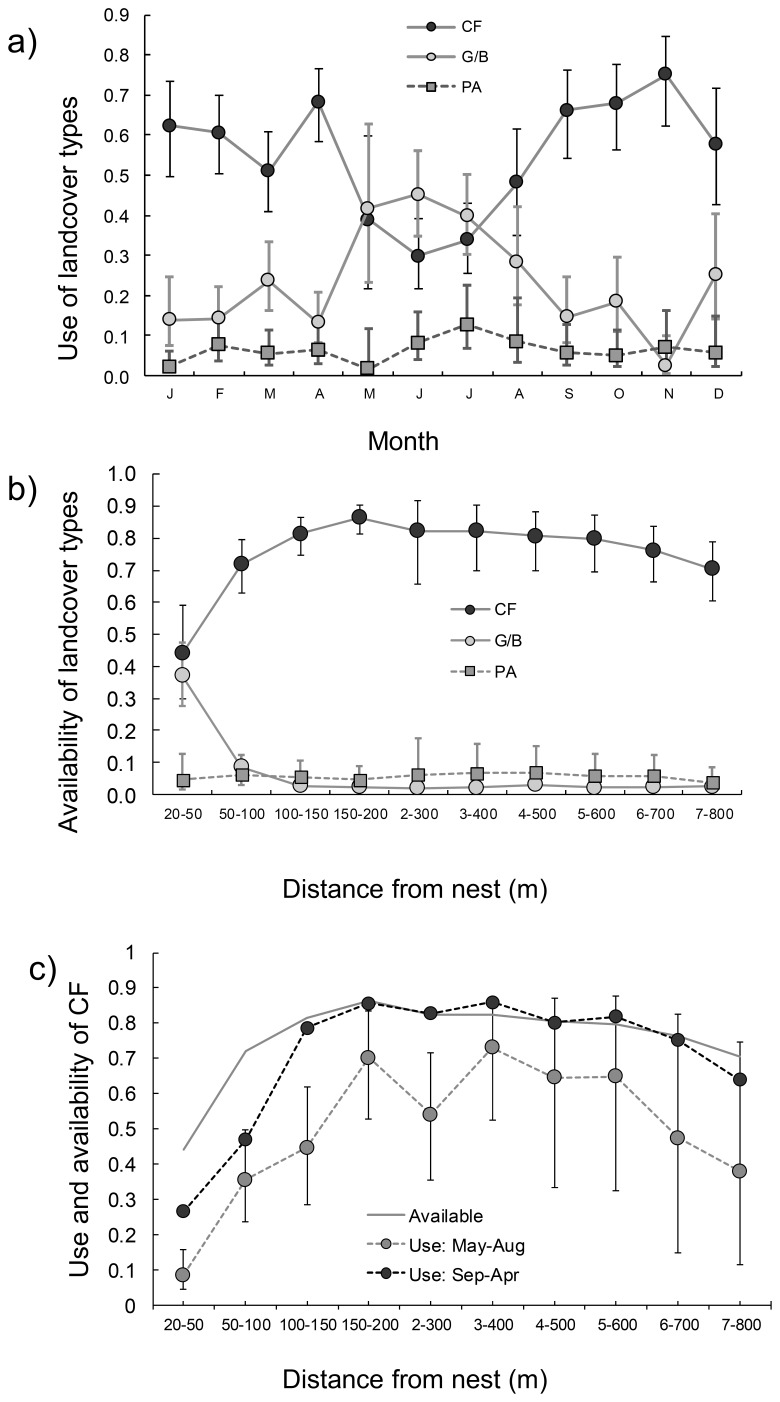
Despite the dynamic nature of habitat selection, temporal variation as arising from factors such as weather are rarely quantified in species-habitat relationships. We analysed habitat use and selection (use/availability) of foraging, radio-tagged little owls (Athene noctua), a nocturnal, year-round resident generalist predator, to see how this varied as a function of weather, season and availability. Use of the two most frequently used land cover types, gardens/buildings and cultivated fields varied more than 3-fold as a simple function of season and weather through linear effects of wind and quadratic effects of temperature. Even when controlling for the temporal context, both land cover types were used more evenly than predicted from variation in availability (functional response in habitat selection). Use of two other land cover categories (pastures and moist areas) increased linearly with temperature and was proportional to their availability. The study shows that habitat selection by generalist foragers may be highly dependent on temporal variables such as weather, probably because such foragers switch between weather dependent feeding opportunities offered by different land cover types. An opportunistic foraging strategy in a landscape with erratically appearing feeding opportunities in different land cover types, may possibly also explain decreasing selection of the two most frequently used land cover types with increasing availability.

Figure 1. Nocturnal dispersion of four radio-tagged little owls from two pairs.

Colour codes indicate whether the owls were perching or were located on the ground, as evident from the strength and echo patterns of the radio signals. Concentric lines 20–800 m from the nest/roosting sites indicate the total area with distance intervals within which habitat use and availability was compared.

Figure 2. Variation in use and availability of the land cover categories ‘Cultivated fields’ (CF), ‘Garden/buildings’ (G/B) and ‘Pastures’ (PA) of radio-tagged little owls (least square means with 95% confidence limits).

(a) Use is divided between months. (b) Availability is divided between distance-to-nest intervals. (c) Availability and seasonal use of cultivated fields is divided between distance-to-nest intervals (confidence errors for use in Sep–Apr are not shown for clarity).

Figure 3. Monthly variation in habitat selection of radio-tagged little owls as predicted from Resource selection functions.

A coefficient value of x means that a land cover type is selected exp(x) times more than the reference category. (A) Selection coefficients ‘cultivated fields’ (CF) and ‘pastures’ (PA) relative to ‘gardens/buildings’ (G/B) (Table B in File S2). (B) Selection for ‘ground moisture’ adjusted for month-specific selection of general land cover categories (shown for all four general land cover categories combined [Table B in File S2] and when modelled within CF and PA only [Tables C–E in File S2]). Statistical significances: *: P<0.05, **: P<0.01, ***: P<0.001, ****: P<0.0001).

Figure 4. Amount of variation in use of different land cover categories of radio-tagged little owls explained by individual predictor variables and combinations of variables.

The maximum rescaled R² expresses the amount of explained variation in terms of reduction of deviance, while Somer’s D (with 95% CIs) expresses a model’s ability to correctly classify whether an owl would be located in a given habitat. Statistical significances; ns: not significant, *: P<0.05, **: P<0.01, ***: P<0.001.

Figure 5. Predicted use of different land cover types of radio-tagged little owls as functions of temperature and wind.

The estimates are based on situations where availability at the home range level is equal to the mean for the population (horizontal red dotted lines) and monthly variation is accounted for (see Table B in File S3 for further details). (A) Predicted use of ‘Cultivated Fields’ (CF) as a function of temperature and wind strength shown for February and June. (B) Predicted use of ‘Gardens/buildings’ (G/B) as a function of temperature and wind strength shown for February and June. (C) Predicted use of pastures (PA) as a function of temperature (thin lines show 95% confidence intervals). (D) (C) Predicted use of ‘Moist areas‘ within PA or CF as a function of temperature (thin lines show 95% confidence intervals).

Figure 6. Use of land cover types by radio-tagged little owls in May–August (warm season) and September–April (cold season) plotted/regressed against availability at home range level and within distance-to-nest intervals.

At the home range level, each dot represents the proportion of time (telemetry fixes) one owl spent in the land cover category. Regression lines show back-transformed predictions from logit-transformed response variables regressed on logit-transformed proportional cover values (thin lines indicate 95% confidence zones). Predictions above the line y = x suggest that a land cover type is used more than expected by availability; predictions below the line that it is used less than availability would predict. The state space of graphs for distance-to-nest intervals represents the 98%-mid fraction of the availabilities observed.

References

-
- McLoughlin PD, Morris DW, Fortin D, Vander Wal E, Contasti AL (2010) Considering ecological dynamics in resource selection functions. Journal of Animal Ecology 79: 4–12. - PubMed
- Johnson DH (1980) The Comparison of Usage and Availability Measurements for Evaluating Resource Preference. Ecology 61: 65–71.
- Aebischer NJ, Robertson PA, Kenward RE (1993) Compositional Analysis of Habitat Use from Animal Radio-Tracking Data. Ecology 74: 1313–1325.
Publication types
MeSH terms
LinkOut - more resources
Full Text Sources
Other Literature Sources