When do microcircuits produce beyond-pairwise correlations?

Abstract

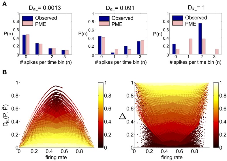
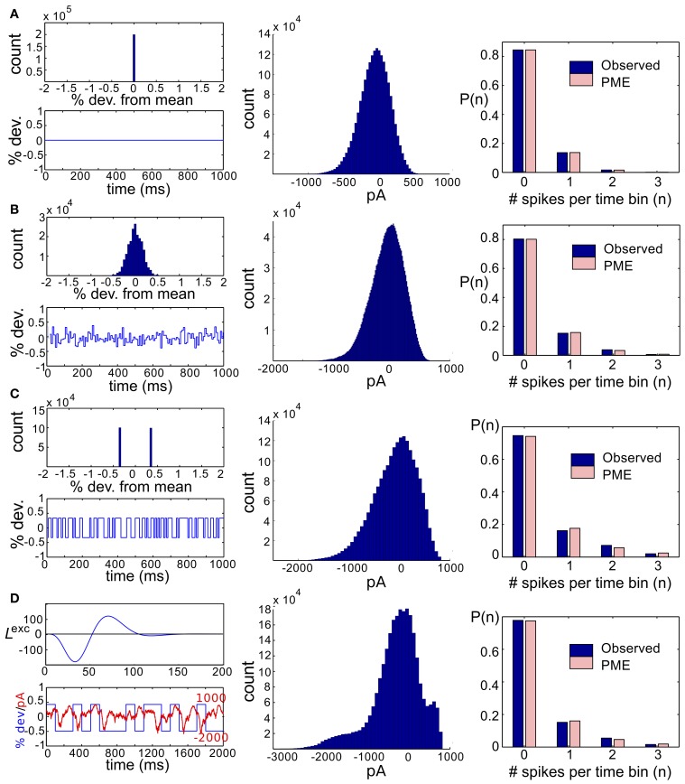
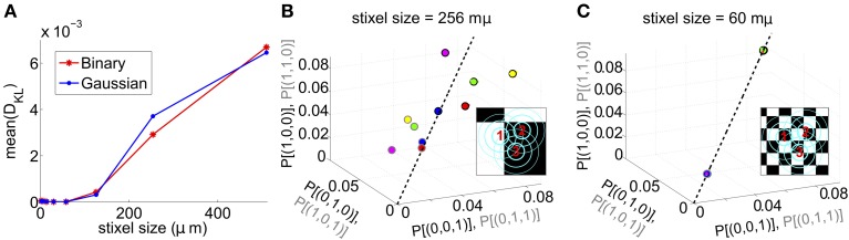
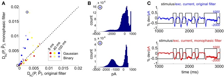
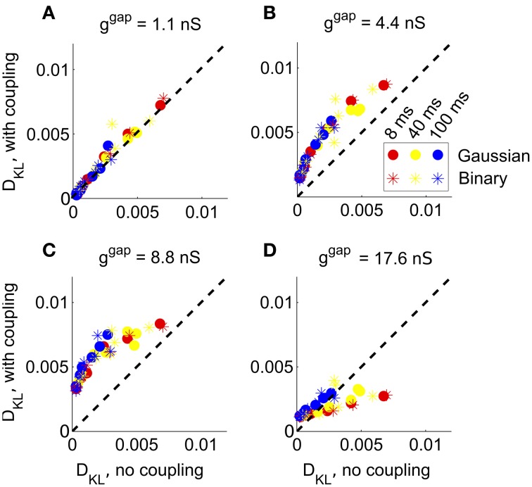
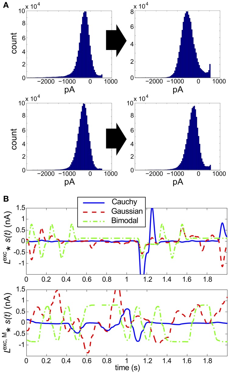
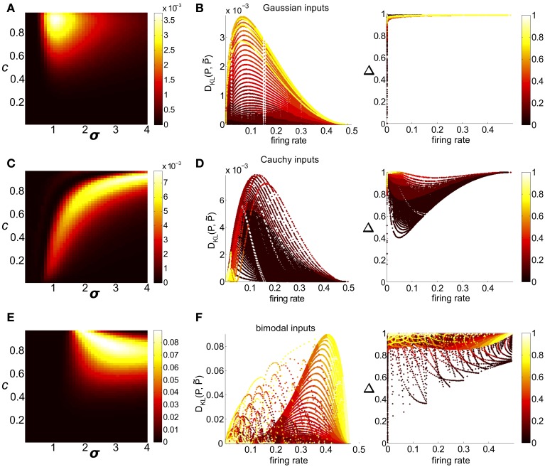
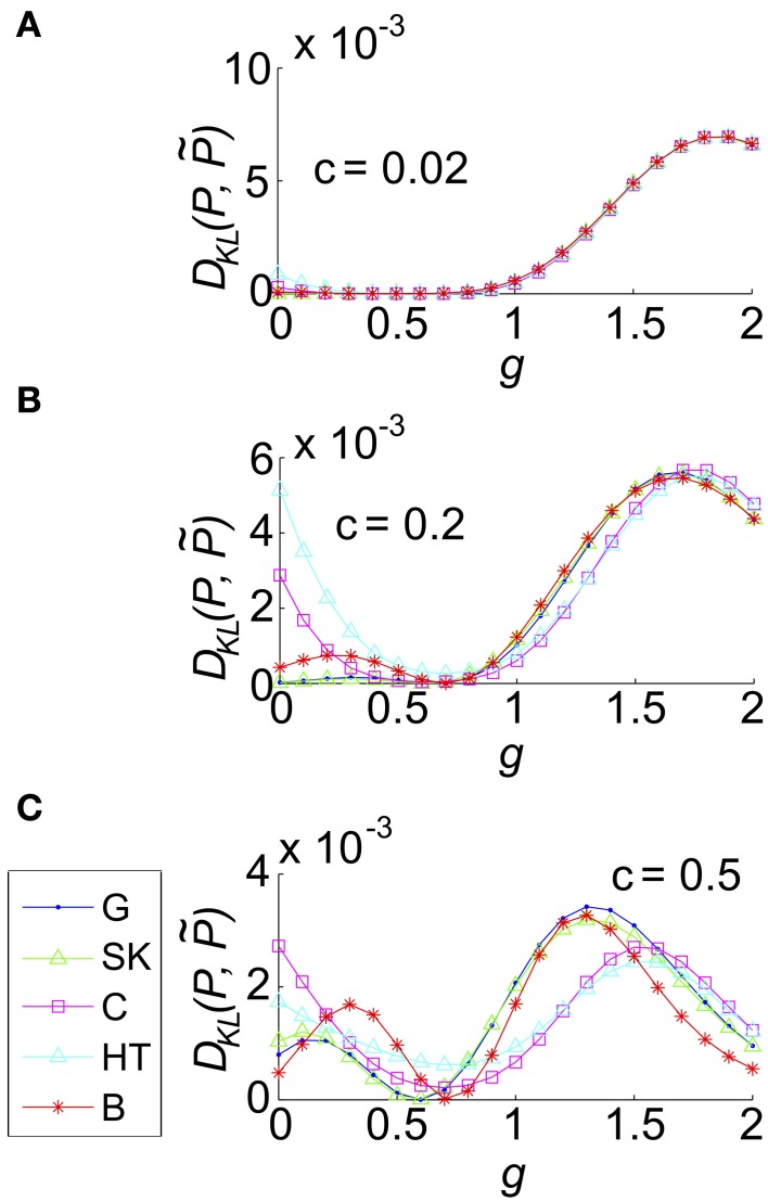
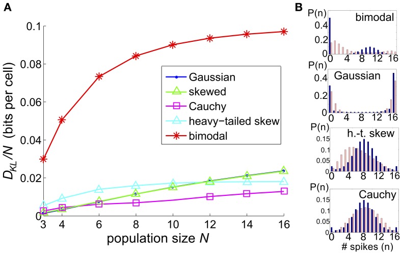
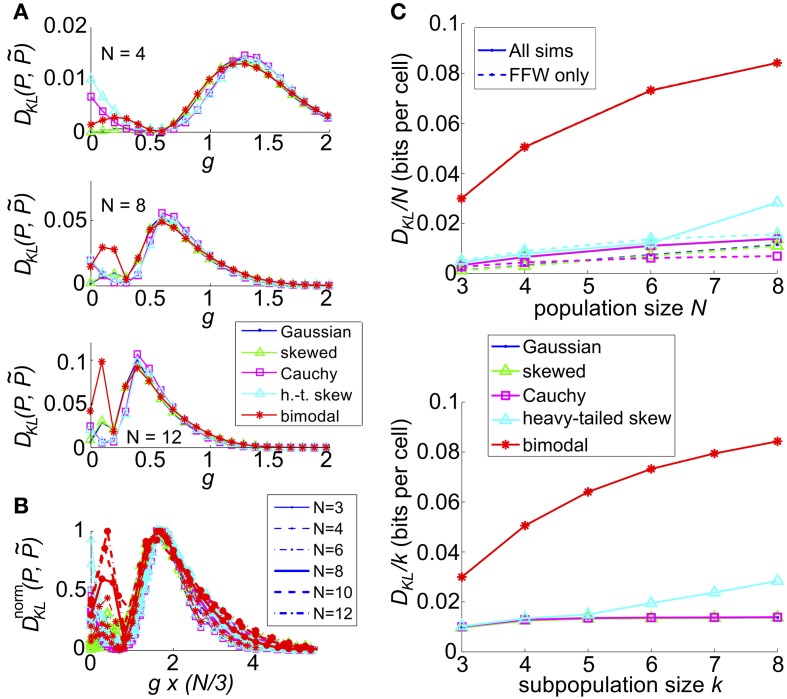
Describing the collective activity of neural populations is a daunting task. Recent empirical studies in retina, however, suggest a vast simplification in how multi-neuron spiking occurs: the activity patterns of retinal ganglion cell (RGC) populations under some conditions are nearly completely captured by pairwise interactions among neurons. In other circumstances, higher-order statistics are required and appear to be shaped by input statistics and intrinsic circuit mechanisms. Here, we study the emergence of higher-order interactions in a model of the RGC circuit in which correlations are generated by common input. We quantify the impact of higher-order interactions by comparing the responses of mechanistic circuit models vs. "null" descriptions in which all higher-than-pairwise correlations have been accounted for by lower order statistics; these are known as pairwise maximum entropy (PME) models. We find that over a broad range of stimuli, output spiking patterns are surprisingly well captured by the pairwise model. To understand this finding, we study an analytically tractable simplification of the RGC model. We find that in the simplified model, bimodal input signals produce larger deviations from pairwise predictions than unimodal inputs. The characteristic light filtering properties of the upstream RGC circuitry suppress bimodality in light stimuli, thus removing a powerful source of higher-order interactions. This provides a novel explanation for the surprising empirical success of pairwise models.

Keywords: computational model; correlations; maximum entropy distribution; retinal ganglion cells; stimulus-driven.

Figure 1

A survey of the quality of the pairwise maximum entropy (PME) model for symmetric spiking distributions on three cells. (A) Probability distribution P (dark blue) and pairwise approximation $\tilde{P}$ (light pink) for three example distributions. From left to right: an example from the simple sum-and-threshold model receiving skewed common input; an example from the sum-and-threshold model receiving bimodal common input [specifically, the distribution with maximal D_KL(P, $\tilde{P}$)]; a specific probability distribution resulting from application of the XOR operator [for illustration of a “worst case” fit of the PME model (Schneidman et al., 2003)]. (B) D_KL(P, $\tilde{P}$) vs. firing rate and Δ vs. firing rate, for a comprehensive survey of possible symmetric spiking distributions on three cells (see text for details). Firing rate is defined as the probability of a spike occurring per cell per random draw of the sum-and-threshold model, as defined in Equation (16). Color indicates output correlation coefficient ρ ranging from black for ρ ∈ (0, 0.1), to white for ρ ∈ (0.9, 1), as illustrated in the color bars.

Figure 2

Results for RGC simulations with constant light and full-field flicker. (A–C) (Left) A histogram and time series of stimulus, (center) a histogram of excitatory conductances and (right) the resulting distribution of spiking patterns. Stimuli are shown as deviations from a baseline intensity, expressed as a fraction of the baseline. Right panels show the probability distribution on spiking patterns P obtained from simulation (“Observed”; dark blue), and the corresponding pairwise approximation $\tilde{P}$ (“PME”; light pink). Each row gives these results for a different stimulus condition. (A) No stimulus (Gaussian noise only). (B) Gaussian input, standard deviation 1/6, refresh rate 8 ms. (C) Binary input, standard deviation 1/3, refresh rate 8 ms. (D) Binary input, standard deviation 1/3, refresh rate 100 ms. For panel (D), the data in the left panel differs. (Left, top panel) The excitatory filter L^exc(t) (Equation 7) is shown instead of a stimulus histogram; (Left, bottom panel) the normalized excitatory conductance, as a function of time (red dashed line), is superimposed on the stimulus (blue solid). (Center) The histogram of excitatory conductances and (right) the resulting distribution of spiking patterns. Both the form of the filter and the conductance trace illustrate that the LN model that processes light input acts as a (time-shifted) high pass filter.

Figure 3

Results for RGC simulations with light stimuli of varying spatial scale (“stixels”). (A) Average D_KL(P, $\tilde{P}$) as a function of stixel size. Values were averaged over five stimulus positions, each with a different (random) stimulus rotation and translation; 512 μm corresponds to full-field stimuli. For the rest of the panels, data from the binary light distributions is shown; results from the Gaussian case are similar. (B,C) Probability of singlet and doublet spiking events, under stimulation by movies of 256 μm (B) and 60 μm (C) stixels. Event probabilities are plotted in 3-space, with the x, y, and z axes identifying the singlet (doublet) events 001 (011), 010 (101), and 100 (110), respectively. The black dashed line indicates perfect cell-to-cell homogeneity (e.g., P[(1, 0, 0)] = P[(0, 1, 0)] = P[(0, 0, 1)]). Both individual runs (dots) and averages over 20 runs (large circles) are shown, with averages outlined in black (singlet) and gray (doublet). Different colors indicate different stimulus positions. Insets: contour lines of the three receptive fields (at the 1 and 2 SD contour lines for the receptive field center; and at the zero contour line) superimposed on the stimulus checkerboard (for illustration, pictured in an alternating black/white pattern).

Figure 4

Comparison of RGC simulations computed with the original ON parasol filter, vs. simulations using a more monophasic filter. (A) D_KL(P, $\tilde{P}$) for original vs. monophasic filter. Data is organized by stimulus refresh rate (8, 40, and 100 ms) and marginal statistics (Gaussian vs. binary). (B) Histograms of excitatory conductances for an illustrative stimulus class, under original (top) and monophasic (bottom) filters. The marginal statistics and refresh rate are illustrated by icons inside black circles; here, binary stimuli with refresh rate 100 ms. The input standard deviation (expressed as a fraction of baseline light intensity) was 1/2. (C) Time course of stimulus and resulting excitatory conductances, from simulation shown in (B): original (top) vs. monophasic (bottom) filters.

Figure 5

The impact of recurrent coupling on RGC networks with full-field visual stimuli. The strength of gap junction connections was varied from a baseline level (relative magnitude g = 1, or absolute magnitude g^gap = 1.1 nS) to an order of magnitude larger (g = 16, or g^gap = 17.6 nS). In each panel, D_KL(P, $\tilde{P}$) obtained with coupling is plotted vs. the value obtained for the same stimulus ensemble without coupling, for each of 42 different stimulus ensembles. (A) g^gap = 1.1 nS (experimentally observed value); (B) g^gap = 4.4 nS; (C) g^gap = 8.8 nS; (D) g^gap = 17.6 nS.

Figure 6

Results for RGC simulations with heavy-tailed inputs. (A) Histograms of excitatory conductances, for the original (left) vs. monophasic (right) filter. The marginal statistics are heavy-tailed skew (top) and Cauchy (bottom) inputs, and refresh rate is 40 ms for both panels. The input standard deviation (expressed as a fraction of baseline light intensity) was 1/2 for both simulations. (B) Sample 100 ms stimuli, filtered by the original linear filter L_exc (top) and altered, monophasic filter L_exc,M(bottom). Cauchy (blue solid), Gaussian (red dashed), and bimodal (green dash-dotted) stimuli are shown.

Figure 7

Strength of higher-order interactions produced by the threshold model as input parameters vary, and the relationship of these higher-order interactions with other output firing statistics. (A) For Gaussian common inputs: D_KL(P, $\tilde{P}$) as a function of input correlation c and input standard deviation σ, for a fixed threshold Θ = 1.5. Color indicates D_KL(P, $\tilde{P}$); see color bar for range. (B) For Gaussian common inputs: D_KL(P, $\tilde{P}$) vs. firing rate (Left) and the fraction of multi-information (Δ) captured by the PME model vs. firing rate (Right). Each dot represents the value obtained from a single choice of the input parameters c, σ, and Θ; input parameters were varied over a broad range as described in section 2. Firing rate is defined as the probability of a spike occurring per cell per random draw of the sum-and-threshold model, as defined in Equation (16). Color indicates output correlation coefficient ρ ranging from black for ρ ∈ (0, 0.1), to white for ρ ∈ (0.9, 1), as illustrated in the color bars. (C,D): as in (A,B), but for Cauchy common inputs. (E,F): as in (A,B), but for bimodal common inputs.

Figure 8

The impact of recurrent coupling on the three-cell sum-and-threshold model. Each plot shows D_KL(P, $\tilde{P}$) as a function of g, for a specific value of the correlation coefficient. In all panels, input standard deviation σ = 1, threshold Θ = 1.5, N = 3 and symbols are as described in the legend for (C). Abbreviations in the legend denote the marginal distribution of the common input: G, Gaussian; SK, skewed; C, Cauchy; HT, heavy-tailed skewed; B, bimodal. (A) For input correlation c = 0.02, (B) c = 0.2, and (C) c = 0.5.

Figure 9

The significance of higher-order interactions increases with network size. (A) Normalized maximal deviation, D_KL(P, $\tilde{P}$)/N, from the PME fit for the thresholding circuit model as network size N increases. For each N and common input distribution type, possible input parameters were in the following ranges: input correlation c ∈ [0, 1], input standard deciation σ ∈ [0, 4], and threshold Θ ∈ [0, 3]. (B) Example sample distributions for different types of common input: from top, bimodal, Gaussian, heavy-tailed skew, and Cauchy common inputs. For each input type, the distribution that maximized D_KL(P, $\tilde{P}$) for N = 16 is shown. Each distribution is illustrated with a bar plot contrasting the probabilities of spiking events in the true (dark blue) vs. pairwise maximum entropy (light pink) distributions.

Figure 10

The impact of recurrent coupling on the sum-and-threshold model, for increasing population size. (A) D_KL(P, $\tilde{P}$) as a function of the coupling coefficient, g, for a specific value of population size N. In all plots, input standard deviation σ = 1, threshold Θ = 1.5 and input correlation c = 0.2. From top: N = 4; N = 8; N = 12. (B) D^norm_KL(P, $\tilde{P}$) as a function of the coupling coefficient, g, for populations sizes N = 3-12. For each curve, D_KL(P, $\tilde{P}$) was scaled by its maximal value and plotted as a function of the scaled coupling coefficient, g^*N/3, to illustrate a universal scaling with effective coupling strength. The line style of each curve indicates the population size N, as listed in the legend. The marker and line color indicate the common input marginal, as listed in the legend for (A). (C) (Top) Maximal value of D_KL(P, $\tilde{P}$)/N, achieved over a survey of parameter values c, σ, Θ, and g, as a function of the population size N (solid lines). For each input marginal type, a second curve shows the maximal value obtained over only feed-forward simulations (g = 0; dashed lines). The marker and line color indicate the common input marginal, as listed in the legend for (A). (Bottom) Maximal value of D_KL(P, $\tilde{P}$)/k, achieved over a survey of parameter values c, σ, Θ, and g, as a function of the subsample population size k. Data was subsampled from the N = 8 data shown in the top panel, by restricting analysis to k out of N cells.

References

1. Amari S. (2001). Information geometry on hierarchy of probability distributions. IEEE Trans. Inf. Theory 47, 1701–1711 10.1109/18.930911 - DOI
1. Amari S., Nakahara H., Wu S., Sakai Y. (2003). Synchronous firing and higher-order interactions in neuron pool. Neur. Comp. 15, 127–142 10.1162/089976603321043720 - DOI - PubMed
1. Badel L., Lefort S., Berger T. K., Petersen C. C. H., Gerstner W., Richardson M. J. E. (2008). Extracting non-linear integrate-and-fire models from experimental data using dynamic I–V curves. Biol. Cybern. 99, 361–370 10.1007/s00422-008-0259-4 - DOI - PMC - PubMed
1. Badel L., Lefort S., Brette R., Petersen C. C. H., Gerstner W., Richardson M. J. E. (2007). Dynamic I-V curves are reliable predictors of naturalistic pyramidal-neuron voltage traces. J. Neurophys. 99, 656–666 10.1152/jn.01107.2007 - DOI - PubMed
1. Barreiro A. K., Shea-Brown E. T., Thilo E. L. (2010). Timescales of spike-train correlation for neural oscillators with common drive. Phys. Rev. E 81, 011916 10.1103/PhysRevE.81.011916 - DOI - PubMed