Fisher's geometrical model emerges as a property of complex integrated phenotypic networks

Abstract

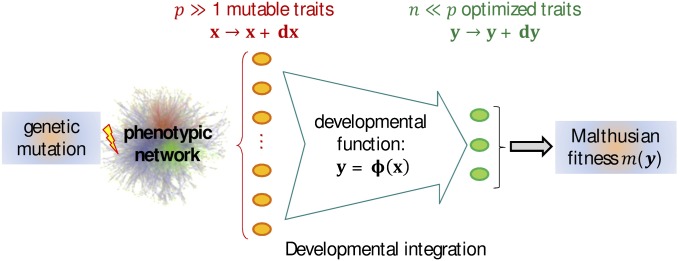
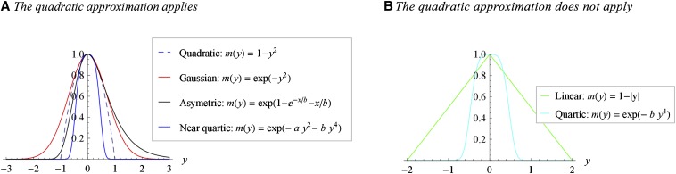
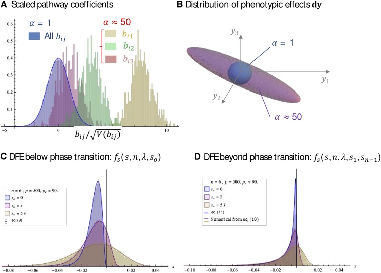
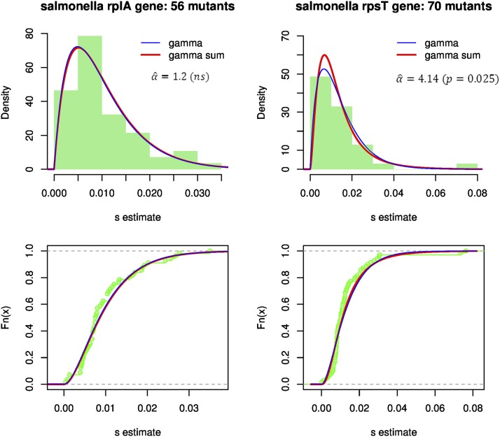
Models relating phenotype space to fitness (phenotype-fitness landscapes) have seen important developments recently. They can roughly be divided into mechanistic models (e.g., metabolic networks) and more heuristic models like Fisher's geometrical model. Each has its own drawbacks, but both yield testable predictions on how the context (genomic background or environment) affects the distribution of mutation effects on fitness and thus adaptation. Both have received some empirical validation. This article aims at bridging the gap between these approaches. A derivation of the Fisher model "from first principles" is proposed, where the basic assumptions emerge from a more general model, inspired by mechanistic networks. I start from a general phenotypic network relating unspecified phenotypic traits and fitness. A limited set of qualitative assumptions is then imposed, mostly corresponding to known features of phenotypic networks: a large set of traits is pleiotropically affected by mutations and determines a much smaller set of traits under optimizing selection. Otherwise, the model remains fairly general regarding the phenotypic processes involved or the distribution of mutation effects affecting the network. A statistical treatment and a local approximation close to a fitness optimum yield a landscape that is effectively the isotropic Fisher model or its extension with a single dominant phenotypic direction. The fit of the resulting alternative distributions is illustrated in an empirical data set. These results bear implications on the validity of Fisher's model's assumptions and on which features of mutation fitness effects may vary (or not) across genomic or environmental contexts.

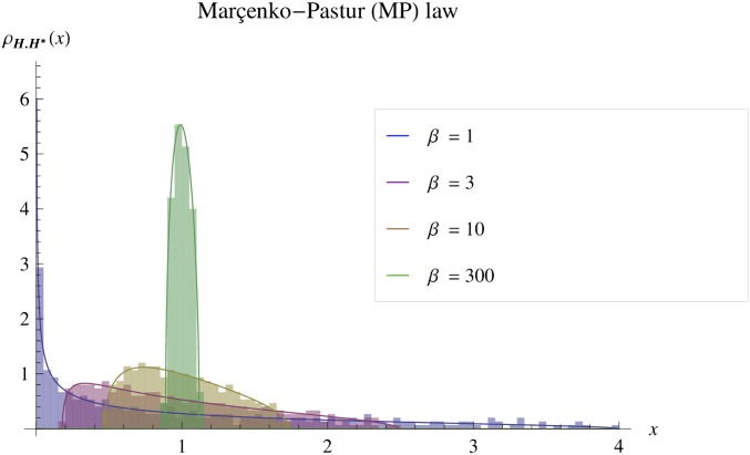
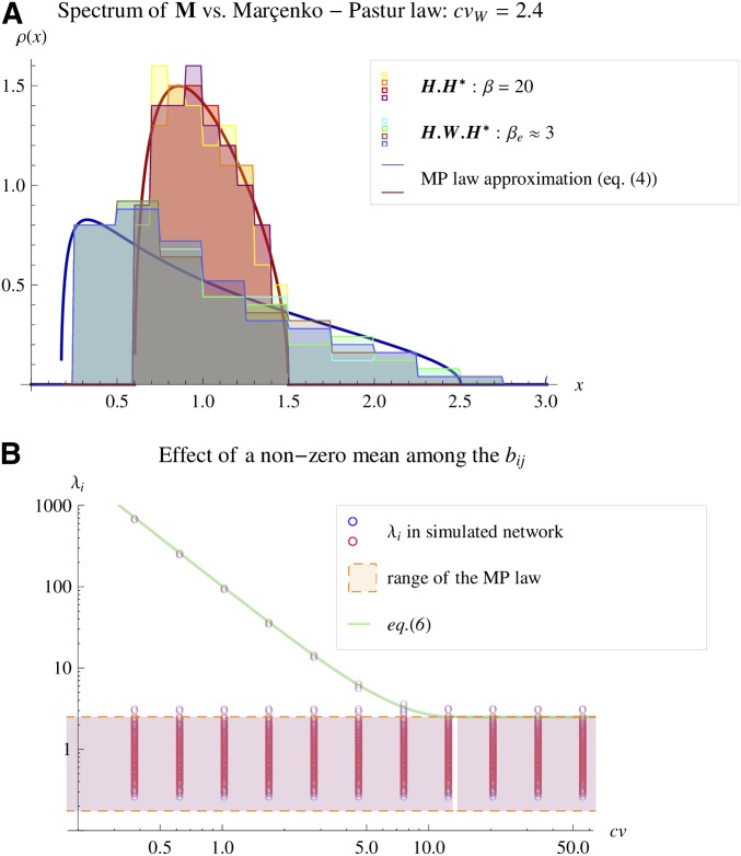
Keywords: Fisher’s geometrical model; mutation fitness effects; network biology; random matrix theory; systems biology.

Figure 1

Model of genotype–phenotype–fitness map. This schematic representation shows the different levels of integration assumed in the model, from a single genetic change in the DNA (left) to its effect on the Malthusian fitness of the whole organism. Each mutation pleiotropically affects a large subset of p “mutable traits” (orange ovals), via a complex interaction network among proteins. The parent phenotype at all these traits is represented by the vector x. The effect of a mutation (on the offspring’s phenotype) is a random small perturbation $dx$ with mean zero and arbitrary multivariate distribution (covariance V). These basic mutational changes “percolate” through the network of interactions to induce changes at a much smaller set of n key integrative traits (“optimized traits,” green ovals), which are those under stabilizing selection, represented by the vector y. An arbitrary developmental function $y=\mathbf{\phi }(x)$ relates mutable to optimized traits (developmental integration). The effect of mutations on y is a perturbation vector $dy$ that is approximately linear in $dx$ (to leading order), with linear coefficients $b_{ij}={\partial }_{x_j}\phi (y_i)$, arbitrarily distributed. The optimized traits directly determine fitness via a locally quadratic function $m(y)$ around some optimum (set at $y=0$).

Figure 2

Applicability of the quadratic approximation around the optimum, for various fitness functions. Different fitness functions $m\left(y\right)$ (indicated in inset) are illustrated in one dimension ($y\in \mathrm{ℝ}$). Conditional on the existence of a nonvanishing second derivative at the optimum ($m^{″}\left(0\right)\ne 0$), the quadratic approximation (dashed line) applies (A) or does not apply (B).

Figure 3

Convergence of the Marchenko–Pastur law toward isotropy. The pdf $\rho (x)$ of the Marchenko–Pastur (M-P) law is illustrated for a set of values of the shape parameter $\beta =p/n$ (see inset). The matrices are scaled to have $E\left(\lambda \right)=1$ ($\zeta =1/\beta$). The histograms show the spectral distribution of a simulated Wishart matrix ($n=300,\beta =p/n$), and the lines show the limit spectral distribution given by the corresponding Marchenko–Pastur law $\lambda \sim \text{MP}(\beta ,1/\beta )$ (Equation 3). The spectral distribution is well captured by the M-P law and becomes narrower as the ratio index becomes larger ($n\ll p$, high integration).

Figure 4

Spectral distributions under the random phenotypic network model. The observed distribution of eigenvalues of M (spectral distribution) is shown together with the predicted M-P law approximation. In each case, a single random phenotypic network (matrices $H, B$, and V) was drawn and the resulting spectral distribution of $H.W.H*$ is shown. The $n\times p$ matrix of pathway coefficients $B={\left\{b_{ij}\right\}}_{i\in \left[1,n\right],j\in [1,p]}$ was set to have mean vector ${\mu }_B={\left\{{\mu }_j\right\}}_{j\in [1,p]}$ drawn randomly with ${\mu }_j~N(0,\sigma )$ and $p\times p$ covariance matrix $C_B$. The pathway coefficients $b_{ij}$ were drawn from various alternative distributions: discrete bimodal $(\pm 1/\sqrt{n})$, normal, uniform, or a mixture of the two. The covariance matrices $C_B \text{and} V$ were drawn independently as Wishart deviates: $V,C_B~W_{p+1}({\Lambda }_p)/(p+1)$, where ${\Lambda }_p$ is a diagonal matrix. The matrix ${\Lambda }_p$ has p gamma-distributed diagonal entries, thus allowing us to set a high coefficient of variation (${\text{cv}}_W$) (A) of the eigenvalues of W (i.e., of $n C_B.V$). The matrices were scaled so that $E\left({\lambda }_{i\ne 1}\right)=1$ in the bulk and the dimensions were $n=100$ and $p=2000.$ A shows the resulting distribution of the bulk eigenvalues ${\lambda }_{i\ne 1}$ of either $H.H*$ or $H.W.H*$ (see inset) and the corresponding M-P law as solid lines. Each histogram color corresponds to a distinct distribution of the $b_{ij}$. B shows the behavior of the dominant eigenvalue ${\lambda }_1$. The coefficient cv (Equation 5) is set in the simulations via the scaling parameter σ. For each value of cv on the x-axis, the full set of eigenvalues is represented by the circles. Red and blue circles correspond to $b_{ij}$ drawn from normal or uniform distributions (undistinguishable). The range of the bulk (${\lambda }_{i\ne 1}$, orange area) and the dominant eigenvalue ${\lambda }_1$ (green line) are well predicted by the M-P law approximation.

Figure 5

Simulated DFE vs. isotropic approximation(s). The distribution of selection coefficients among random mutations is represented for different situations (see File S3). The network was simulated as in Figure 4. The bias μ_B${\mu }_B$ was scaled to obtain a given level of α: $\alpha =1$ (C) or $\alpha =50$ (D). The mutable traits $dx$ were drawn as i.i.d. uniform deviates and scaled to obtain $V\left(dx\right)=V$. Then $dy=B.dx$ was computed and scaled to enforce $E\left(s\right)=-\mathrm{0.01.}$ The n parental coordinates $y_i$ were drawn as standard normal deviates and scaled to enforce a given ${\Vert y\Vert }^2/2=s_{\text{o}}$. The fitness effect of mutations was then computed from y and $dy$ according to Equation 1. All other parameters are indicated in the insets: $n=6, p=200.$ A illustrates the distribution of pathway coefficients, scaled by their variance ($b_{ij}/\sqrt{V(b_{ij})}$) for each situation: below the phase transition [$\alpha =1$: all $b_{ij}$ under the same blue histogram $N(0,1)$] or beyond the phase transition ($\alpha =50$: each color gives the $b_{ij}$ for a given index j for the three first mutable traits). The corresponding anisotropy in the spectral distribution of M is illustrated in B: ellipsoids are the 95% domain of the mutant phenotypes on the three first optimized traits $y_i$. Beyond the phase transition ($\alpha =50$: purple cloud), there is a favored direction in y space. C and D show the corresponding DFE, below (C) or beyond (D) the phase transition, at the optimum ($s_{\text{o}}=0$, blue), close to it ($s_{\text{o}}=\overline{s}$, red), or farther from it ($s_{\text{o}}=5 \overline{s}$, brown). The lines show the corresponding analytic predictions [Equation 9 (C) or Equations 10 and 11 (D)] (see insets).

Figure 6

Fit of the gamma and gamma sum models to empirical DFEs in bacteria. Top, the distribution of selection coefficients among random nucleotide substitutions vs. alternative fitted models: Equation 11 with $\alpha =1$ (a gamma distribution, blue curve) or α freely fitted (a convolution of two gammas, red curve). Bottom, the corresponding empirical cumulative distribution function vs. fitted models. The values of the best-fit parameters are given in Table 2. The significance of the test for $\alpha >1$ vs. $\alpha =1$ is given below the estimated value.

References

-
- Bai Z., Silverstein J. W., 2010. Spectral Analysis of Large Dimensional Random Matrices, Ed. 2. now Publishers Inc., Hanover, MA.
- Barabasi A. L., Oltvai Z. N., 2004. Network biology: understanding the cell’s functional organization. Nat. Rev. Genet. 5: 101–113. - PubMed
- Barton N. H., Coe J. B., 2009. On the application of statistical physics to evolutionary biology. J. Theor. Biol. 259: 317–324. - PubMed
- Bataillon T., 2000. Estimation of spontaneous genome-wide mutation rate parameters: Whither beneficial mutations? Heredity 84: 497–501. - PubMed
- Baxter G. J., Blythe R. A., McKane A. J., 2007. Exact solution of the multi-allelic diffusion model. Math. Biosci. 209: 124–170. - PubMed
Publication types
MeSH terms
LinkOut - more resources
Full Text Sources
Other Literature Sources
Miscellaneous