Estimating dose painting effects in radiotherapy: a mathematical model

Abstract

Tumor heterogeneity is widely considered to be a determinant factor in tumor progression and in particular in its recurrence after therapy. Unfortunately, current medical techniques are unable to deduce clinically relevant information about tumor heterogeneity by means of non-invasive methods. As a consequence, when radiotherapy is used as a treatment of choice, radiation dosimetries are prescribed under the assumption that the malignancy targeted is of a homogeneous nature. In this work we discuss the effects of different radiation dose distributions on heterogeneous tumors by means of an individual cell-based model. To that end, a case is considered where two tumor cell phenotypes are present, which we assume to strongly differ in their respective cell cycle duration and radiosensitivity properties. We show herein that, as a result of such differences, the spatial distribution of the corresponding phenotypes, whence the resulting tumor heterogeneity can be predicted as growth proceeds. In particular, we show that if we start from a situation where a majority of ordinary cancer cells (CCs) and a minority of cancer stem cells (CSCs) are randomly distributed, and we assume that the length of CSC cycle is significantly longer than that of CCs, then CSCs become concentrated at an inner region as tumor grows. As a consequence we obtain that if CSCs are assumed to be more resistant to radiation than CCs, heterogeneous dosimetries can be selected to enhance tumor control by boosting radiation in the region occupied by the more radioresistant tumor cell phenotype. It is also shown that, when compared with homogeneous dose distributions as those being currently delivered in clinical practice, such heterogeneous radiation dosimetries fare always better than their homogeneous counterparts. Finally, limitations to our assumptions and their resulting clinical implications will be discussed.

Figure 1. Cell processes mimicked in the model of tumor growth.

Schematic representation of the cell processes considered in the model of tumor growth (symmetric and asymmetric division, migration, death by radiation, apoptosis (programmed death) and lysis (removal of debris)). Notice that CSCs can perform all these cell processes, while replication of CCs is always supposed to be symmetric. See Document S1 for further details.

Figure 2. Scheme showing the possible actions that a cell is able to perform in the model.

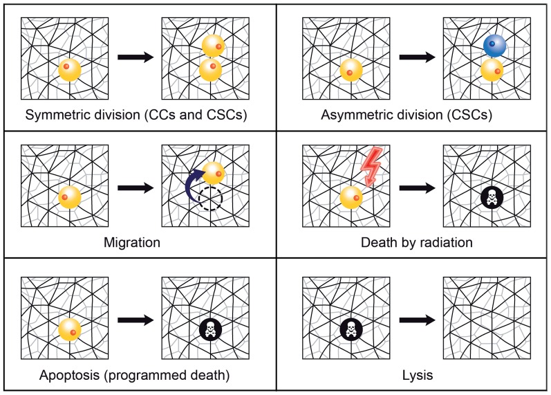
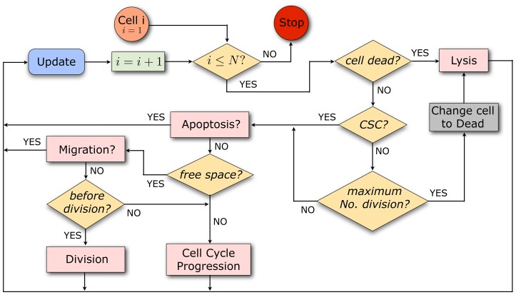
As long as the population size is below a prescribed maximum , it is first tested whether a cell is dead. If so, it undergoes lysis at a certain rate. Alive cells are classified according to CSCs and CCs; CCs die and are subject to lysis with a certain rate once they have performed the maximum number of cell divisions prescribed. CCs not having yet reached the maximum number of cell divisions and CSCs can undergo apoptosis. Those cells that do not go through apoptosis can migrate if free space is available. If they do not migrate and have sufficiently advanced in the cell cycle, they divide. If those cells have not yet reached the end of G2-phase, then they continue to progress in the cell cycle. Cells with no free space available at neighboring sites can only progress in the cell cycle. Concerning radiation effects, cells are picked randomly and killed according to the corresponding surviving cell fraction estimate. See Document S1 for details on the technical implementation of the model algorithm.

Figure 3. Standard radiotherapy treatment in a homogeneous tumor for the low and high migration cases.

Cell growth curves are shown corresponding to homogeneous tumor growth for the low and high migration cases when only CCs are present (see respectively (A) and (C)). Tumor growth is allowed unchecked from a size of about 10⁵ cells until about 10⁶ cells are present, which approximately occurs at day 30 (respectively at day 7) since the beginning of the process. Then, a homogeneous treatment corresponding to 30 sessions of 2.0 Gy each is delivered. In all cases, sessions are scheduled along 6 weeks separated by 24 hours intervals except for weekends, where a 72 hours interval is allowed. Radiotherapy treatment is thus completed 40 days afterwards its beginning (about 70 and 47 days since the initial stage respectively). Data corresponding to 20 simulations (with different seeds of a random number generator) are presented. Notice that the vertical coordinate is represented in a logarithmic scale. In (B) and (D) tumor stages are represented when radiation therapy is started (about 10⁶ cells in total) for the low and high migration cases respectively. Depicted in dark and light green are proliferating and quiescent CCs. Dead cells are represented in black. See Movies S1 and S2 for an example of simulations represented in (A) and (C).

Figure 4. Simulated growth of a heterogeneous tumor with the low migration rate.

Depicted in dark and light green (respectively, dark and light red) are proliferating and quiescent CCs (respectively, proliferating and quiescent CSCs). Dead cells are represented in black. (A) An initial stage where about 10⁵ cells, distributed into tumor cell phenotypes CC (85%) and CSC (15%), are present. (B) Tumor stage when radiation therapy is started (about 10⁶ cells in total). 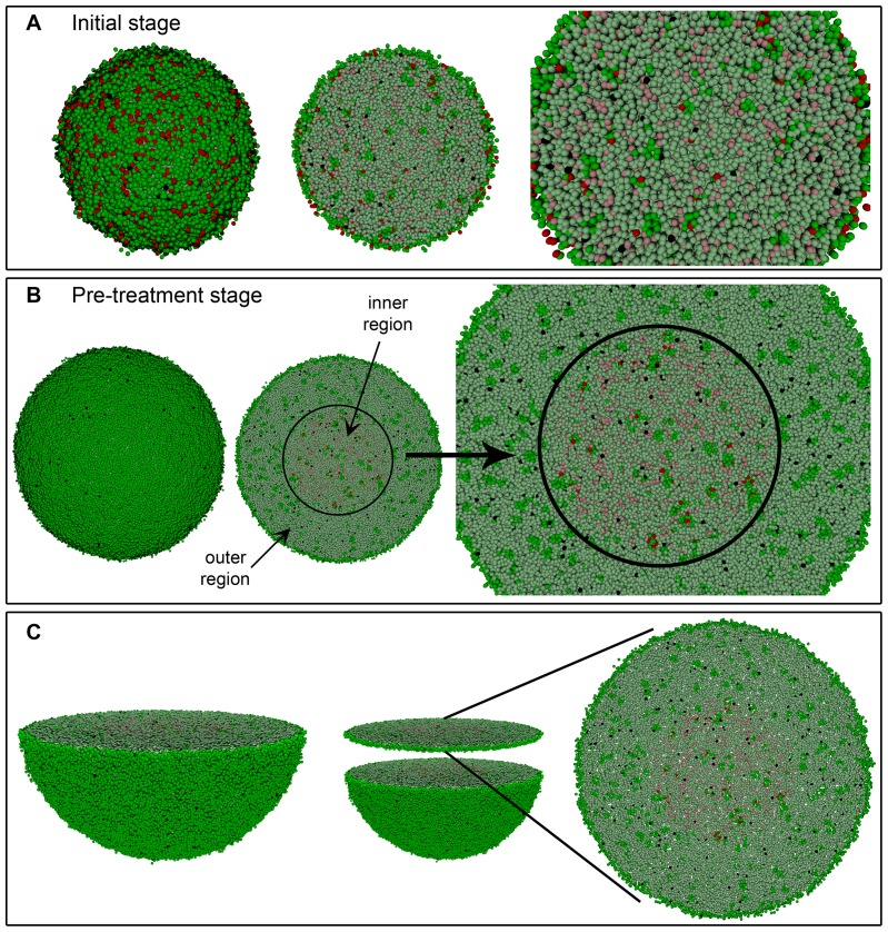In the middle image, the location of the inner region where 100% of CSCs are concentrated is shown for the case when and CSC cycle duration equal to 96 h. A 3D transversal cut is performed in the middle of solid figures (A) and (B) (left), so that its interior could be seen (middle and right) respectively. (C) Representation of the transversal cut showed in (B) for a slice of two cell diameters. Notice the little space existing between cells.

Figure 5. Simulated growth of a heterogeneous tumor with the high migration rate.

Depicted in dark and light green (respectively, dark and light red) are proliferating and quiescent CCs (respectively, proliferating and quiescent CSCs). Dead cells are represented in black. (A) An initial stage where about 10⁵ cells, distributed into tumor cell phenotypes CC (85%) and CSC (15%), are present. (B) Tumor stage when radiation therapy is started (about 10⁶ cells in total). 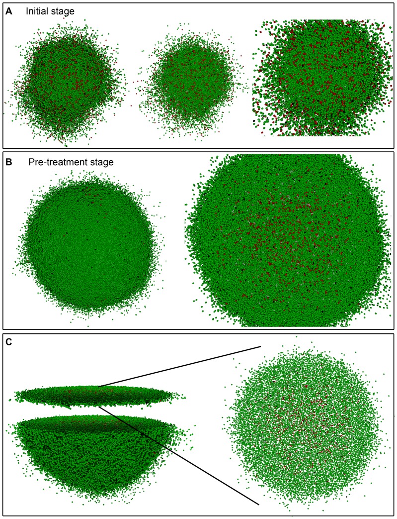In the right image, the spatial distribution of CCs and CSCs is shown for the case when and CSC cycle duration equal to 48 h. A 3D transversal cut is performed in the middle of solid figure (B) (left), so that its interior could be seen (right). (C) Representation of the transversal cut showed in (B) for a slice of two cell diameters. Notice the comparatively large (with respect to Figure 4) space observed between cells.

Figure 6. Spatial distribution of CSCs for a heterogeneous tumor with the high migration rate.

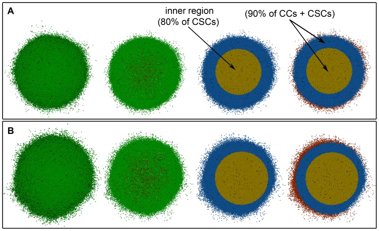
From left to right tumor stage when radiation therapy is started (about 10⁶ cells in total) with the high migration rate, 3D transversal cut in the middle of the tumor, region where 80% of CSCs are located (yellow) and region where 90% of total cells (CCs and CSCs) are located (yellow and blue). (A) For the case and (B) for considering CSC cycle duration equal to 48 h. Depicted in dark and light green (respectively, dark and light red) are proliferating and quiescent CCs (respectively, proliferating and quiescent CSCs). Dead cells are represented in black.

Figure 7. Comparing heterogeneous and averaged homogeneous radiation therapies in a heterogeneous tumor for different model parameters.

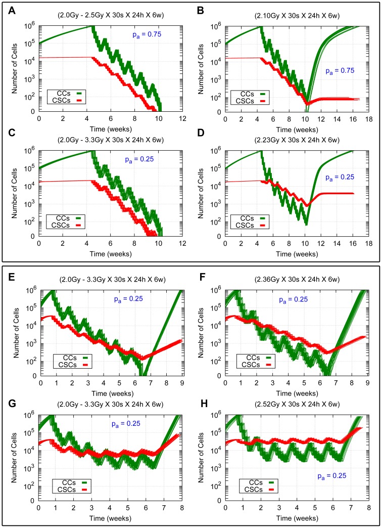
Cell survival curves for 20 simulations (with different seeds of a random number generator) in the cases and for CSC cycle durations equal to 96 h and 48 h with the high and low migration rates are shown. The time evolution for CCs and CSCs is represented in green and red respectively. (A, C, E, G) Results for heterogeneous therapies consisting of 2.5 Gy and 3.3 Gy in the inner sphere and 2.0 Gy in the rest of the tumor. (B, D, F, H) Results for the related averaged homogeneous therapies corresponding to 2.10 Gy, 2.23 Gy, 2.36 Gy and 2.52 Gy respectively. (A, B, C, D) Results for the cases and with the low migration rate and CSC cycle duration equal to 96 h. (E, F, G, H) Results for the case with the high migration rate and CSC cycle durations equal to 93 h (E, F) and 48 h (G, H). In all cases 30 sessions are scheduled along 6 weeks, separated by 24 hours intervals except for weekends, where a 72 hours interval is allowed. Radiation is applied when the total cell count is about 10⁶ cells. Notice that the vertical coordinate is represented in a logarithmic scale. See Movies S3, S4, S7 and S8 for an example of simulations represented in (B), (D), (G) and (H) respectively.

Figure 8. Time evolution of tumor growth during and after averaged homogeneous radiation therapies.

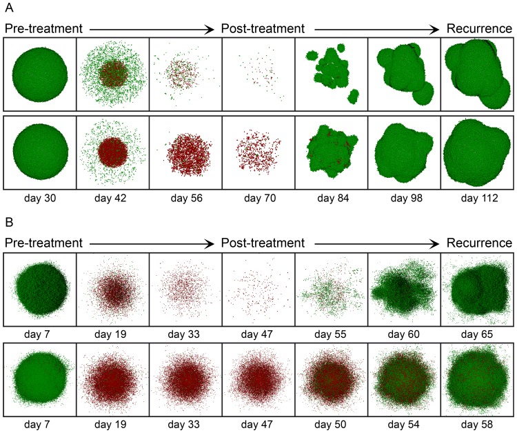
(A) A homogeneous dose of 2.10 Gy for the case is delivered (Top), and a homogeneous dose of 2.23 Gy for is instead applied (Bottom), assuming in both cases of (A) the low migration rate and CSC cycle duration equal to 96 h. (B) A homogeneous dose of 2.36 Gy is delivered (Top) and a homogeneous dose of 2.52 Gy (Bottom) for the case with the high migration rate and CSC cycle durations equal to 96 h (Top) and 48 h (Bottom). In all cases (A, B) a standard scheduling (30 sessions along 6 weeks separated by 24 hours intervals except for weekends) was applied. From left to right we show in sequential order the tumor before radiotherapy treatment starts, its state after sessions 10, 20 and 30, and three stages corresponding to recurrence during the period covered (where about 10⁶ cells is again obtained). Depicted in dark and light green (respectively, dark and light red) are proliferating and quiescent CCs (respectively, proliferating and quiescent CSCs). Dead cells are not represented.

Figure 9. Estimates on the total number of CSCs at the end of the recurrence tumor stage.

Number of CSCs at the end of the recurrence tumor stage (where about 10⁶ cells is again obtained) and the corresponding standard deviations after performing 20 simulations in each case (with different seeds of a random number generator) are shown. 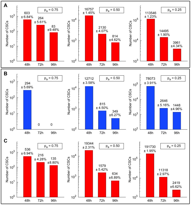(A) For averaged homogeneous therapies corresponding to heterogeneous therapies consisting of 2.5 Gy, 2.9 Gy and 3.3 Gy in the inner sphere and 2.0 Gy in the rest of the tumor for the cases , and (left, middle, right) assuming the low migration rate and CSC cycle durations equal to 48 h, 72 h and 96 h (see Table 4). (B) For heterogeneous therapies consisting of 2.5 Gy, 2.9 Gy and 3.3 Gy in the inner sphere and 2.0 Gy in the rest of the tumor (Top) and the corresponding averaged homogeneous therapies (Bottom) for the cases , and (left, middle, right) with the high migration rate and CSC cycle durations equal to 48 h, 72 h and 93 h (see Table 5). In all cases (A, B, C), a standard scheduling (30 sessions along 6 weeks separated by 24 hours intervals except for weekends) was applied. Notice that the vertical coordinate is represented in a logarithmic scale. See Tables in the Document S1 for further details and Movies S3, S4, S5, S6, S7 and S8 for some examples of simulations represented in (A), (B) and (C).

Figure 10. Comparing averaged homogeneous radiation therapies without weekend interruptions.

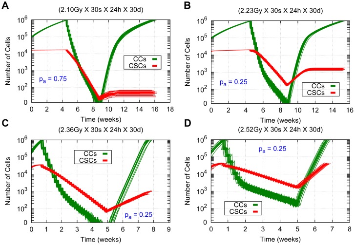
Cell survival curves for 20 simulations (with different seeds of a random number generator) are shown. (A) Averaged dosimetries consisting of for and (B) for , both for the low migration case and CSC cycle duration equal to 96 h. (C, D) Averaged homogeneous therapies consisting of and for the case with the high migration rate and CSC cycle durations equal to 96 h and 48 h respectively. The time evolution of CCs and CSCs are represented in green and red respectively. In all cases (A, B, C, D), sessions were scheduled 7 days a week separated by 24 hours intervals along 30 sessions (without weekend interruptions). Notice that the vertical coordinate is represented in a logarithmic scale. See Movie S9 for an example of simulations represented in (D).

Figure 11. Comparing the effects of lower radiation dosimetries with and without hyperfractionation.

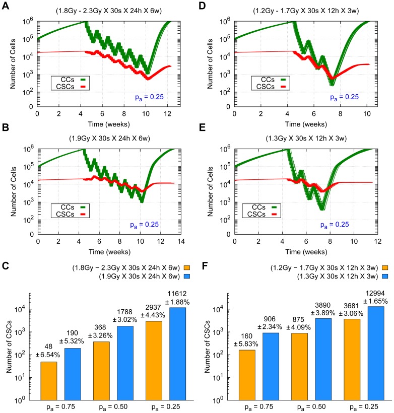
Cell survival curves for 20 simulations (with different seeds of a random number generator) are shown in the case for the low migration case and CSC cycle duration equal to 96 h. (Top) From left to right heterogeneous therapies consisting of 2.3 Gy (A) and 1.7 Gy (D) in the inner sphere, and 1.8 Gy (A) and 1.2 Gy (D) in the rest of the tumor respectively. (Middle) From left to right the averaged homogeneous therapies corresponding to 1.9 Gy (B) and 1.3 Gy (E) are represented. Radiation dose delivery been made according to 5 days a week, 30 sessions in total, at 24 hours (A, B) and at 12 hours (D, E) intervals with weekend interruptions. The time evolution of CCs and CSCs is represented in green and red respectively. (Bottom) Number of CSCs and the corresponding standard deviations at the end of the recurrence tumor stage (where about 10⁶ cells is again obtained) for heterogeneous (yellow) and averaged homogeneous (blue) radiation therapies (C, F). Notice that the vertical coordinate is represented in a logarithmic scale. See Movie S10 for an example of simulations represented in (E).