Stability indicators in network reconstruction

Abstract

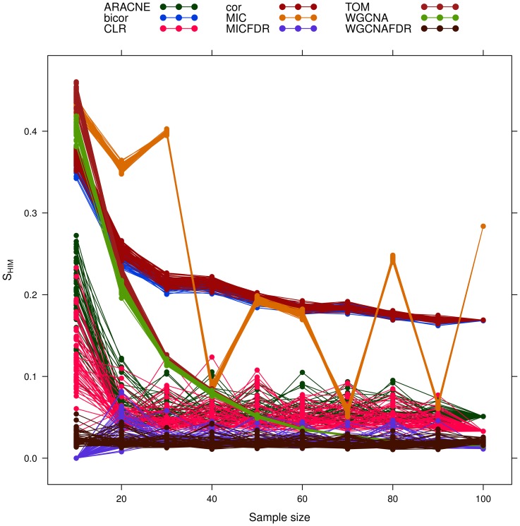
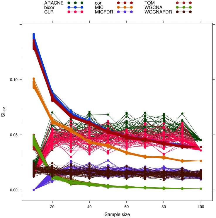
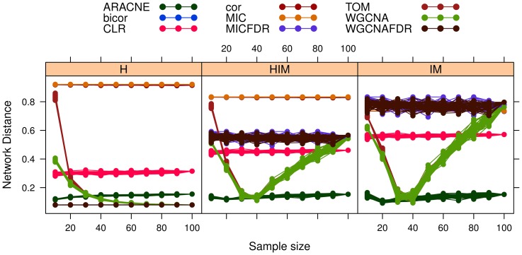
The number of available algorithms to infer a biological network from a dataset of high-throughput measurements is overwhelming and keeps growing. However, evaluating their performance is unfeasible unless a 'gold standard' is available to measure how close the reconstructed network is to the ground truth. One measure of this is the stability of these predictions to data resampling approaches. We introduce NetSI, a family of Network Stability Indicators, to assess quantitatively the stability of a reconstructed network in terms of inference variability due to data subsampling. In order to evaluate network stability, the main NetSI methods use a global/local network metric in combination with a resampling (bootstrap or cross-validation) procedure. In addition, we provide two normalized variability scores over data resampling to measure edge weight stability and node degree stability, and then introduce a stability ranking for edges and nodes. A complete implementation of the NetSI indicators, including the Hamming-Ipsen-Mikhailov (HIM) network distance adopted in this paper is available with the R package nettools. We demonstrate the use of the NetSI family by measuring network stability on four datasets against alternative network reconstruction methods. First, the effect of sample size on stability of inferred networks is studied in a gold standard framework on yeast-like data from the Gene Net Weaver simulator. We also consider the impact of varying modularity on a set of structurally different networks (50 nodes, from 2 to 10 modules), and then of complex feature covariance structure, showing the different behaviours of standard reconstruction methods based on Pearson correlation, Maximum Information Coefficient (MIC) and False Discovery Rate (FDR) strategy. Finally, we demonstrate a strong combined effect of different reconstruction methods and phenotype subgroups on a hepatocellular carcinoma miRNA microarray dataset (240 subjects), and we validate the analysis on a second dataset (166 subjects) with good reproducibility.

Figure 1. HIM distance: contribution of H and IM.

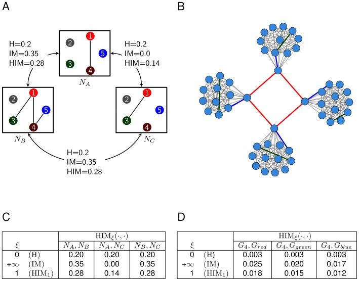
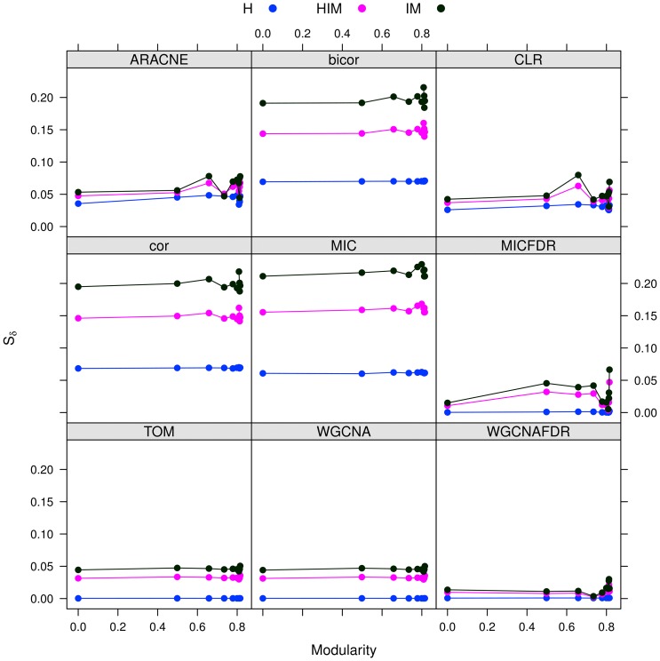
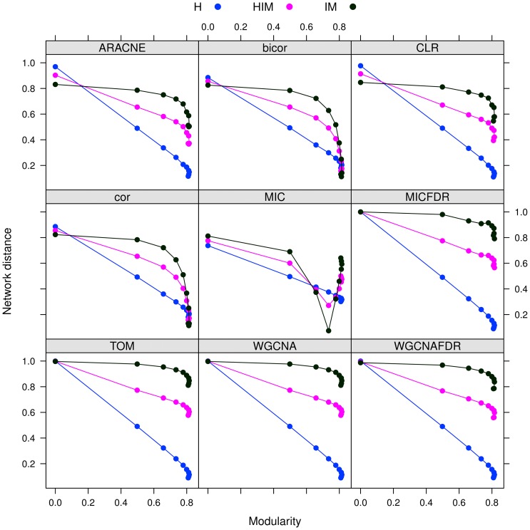
(A) An example on three 5-node networks mutually differing by two links. (B) An example on network , as defined in Subsection Stability is modularity invariant. : network without the four red links. : network without green links. : network without blue links. (C) The mutual differences between the pairs of networks in (A), and . (D) , , . In both cases they have the same Hamming distance but different spectral structure, thus resulting in different Ipsen-Mikhailov distances.

Figure 2. An example of HIM distance.

Representation of the HIM distance in the Ipsen-Mikhailov (IM axis) and Hamming (H axis) distance space between networks A versus B, E and F, where E is the empty network and F is the fully connected one.

Figure 3. Definition of the NetSI family.

Figure 4. Graphical description of the pipeline in Fig. 3.

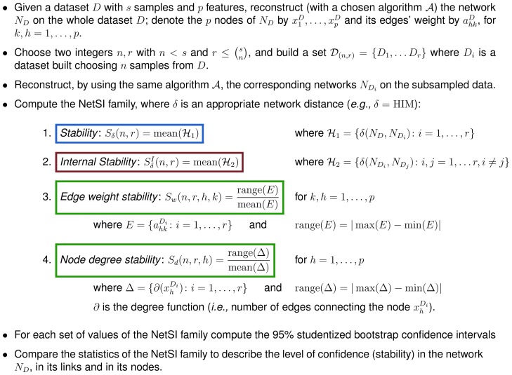
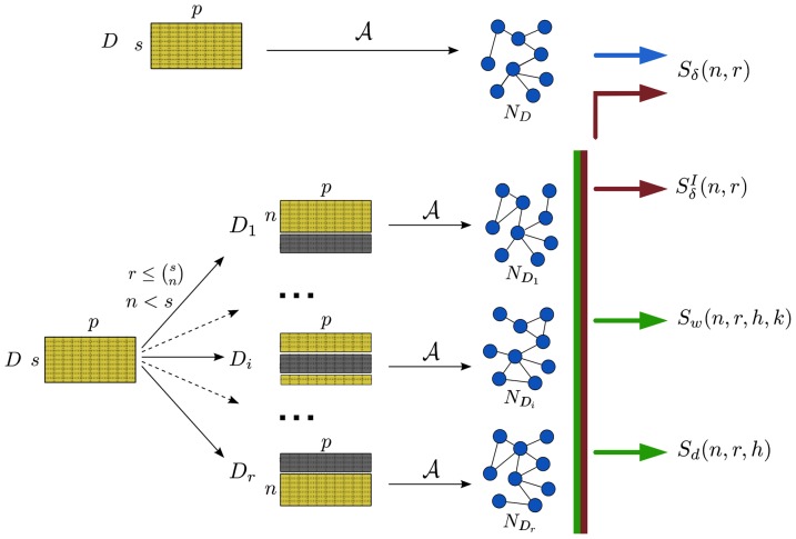
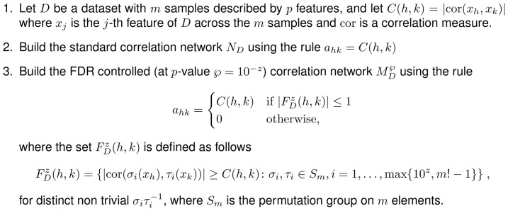
Using the inference algorithm , the network is first reconstructed from the whole dataset with samples and features (nodes). Given two integers , a set of datasets is generated by choosing for each a subset of samples from , and the corresponding networks are inferred by . Finally, the four indicators , , and are computed according to their definition.

Figure 5. Synthetic network with modules, where ranges from 2 to 10 from top left to bottom right.

Figure 6. networks: Stability of synthetic networks for different modularity levels.

Figure 7. networks: distance between gold standard (HIM) and inferred synthetic networks for different modularity levels.

Figure 8. Yeast-like simulated data: effect of increasing sample size on network reconstruction stability .

Different network inference algorithms are compared.

Figure 9. Yeast-like simulated data: effect of increasing sample size on network reconstruction internal stability .

Different network inference algorithms are compared.

Figure 10. Yeast-like simulated data: effect of increasing sample size on network reconstruction accuracy measured as HIM distance and its components Hamming (H) and Ipsen-Mikhailov (IM) with respect to the gold standard.

Different network inference algorithms are compared.

Figure 11. Construction of an FDR-corrected correlation network.

Figure 12. The correlation matrix used to generate the synthetic dataset .

Figure 13. Synthetic dataset : correlation networks inferred by using (A) WGCNA [W], (B) (absolute) Pearson with FDR correction at -value [C()] and (C) MIC [M].

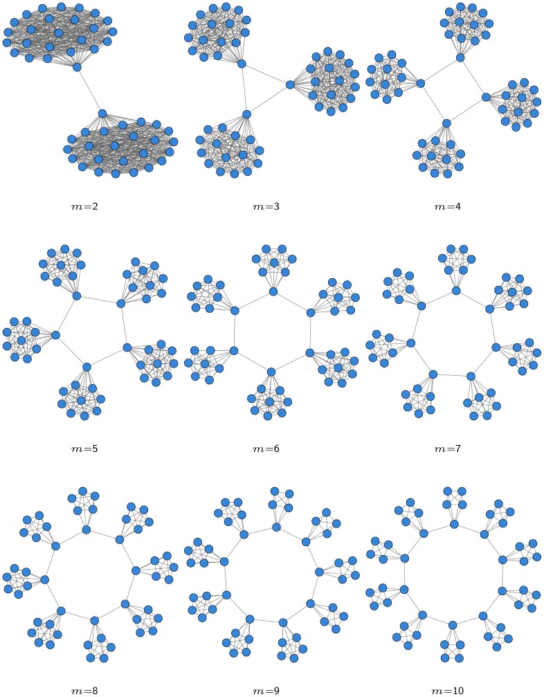
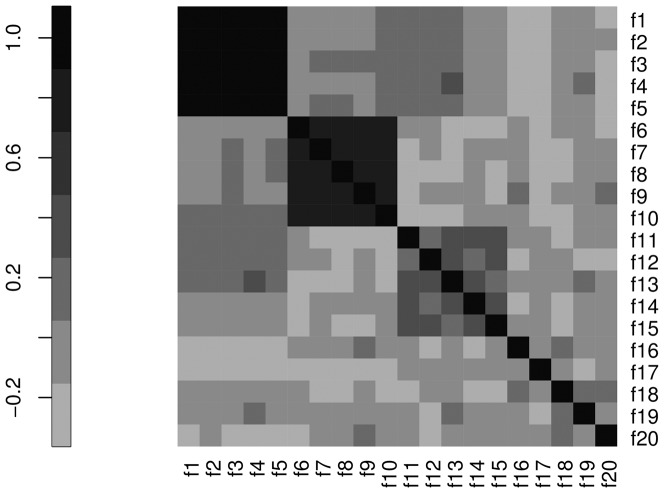
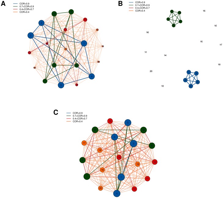
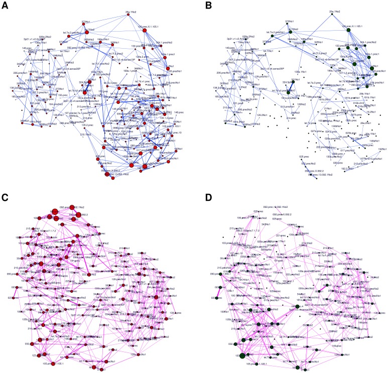
Node label corresponds to feature , node size is proportional to node degree and link colors identify different classes of link weights.

Figure 14. Synthetic dataset : representation of and stability indicators (with confidence intervals) for different instances of the FDR-corrected correlation networks, CORFDR(), CORFDR(), and CORFDR(), WGCNA and MIC networks on the dataset and for different values of data subsampling.

Figure 15. HCC-B dataset: CLR networks in the hairball representation inferred from the 4 subsets (A) Male Tumoral (MT), (B) Male non Tumoral (MnT), (C) Female Tumoral (FT), and (D) Female non Tumoral (FnT).

Links are thresholded at weight 0.1, node position is fixed across the four networks, node dimension is proportional to the degree and edge width is proportional to link weight.

Figure 16. HCC-B dataset: CLR networks in the hiveplot representation inferred from the 4 subsets (A) Male Tumoral (MT), (B) Male non Tumoral (MnT), (C) Female Tumoral (FT), and (D) Female non Tumoral (FnT).

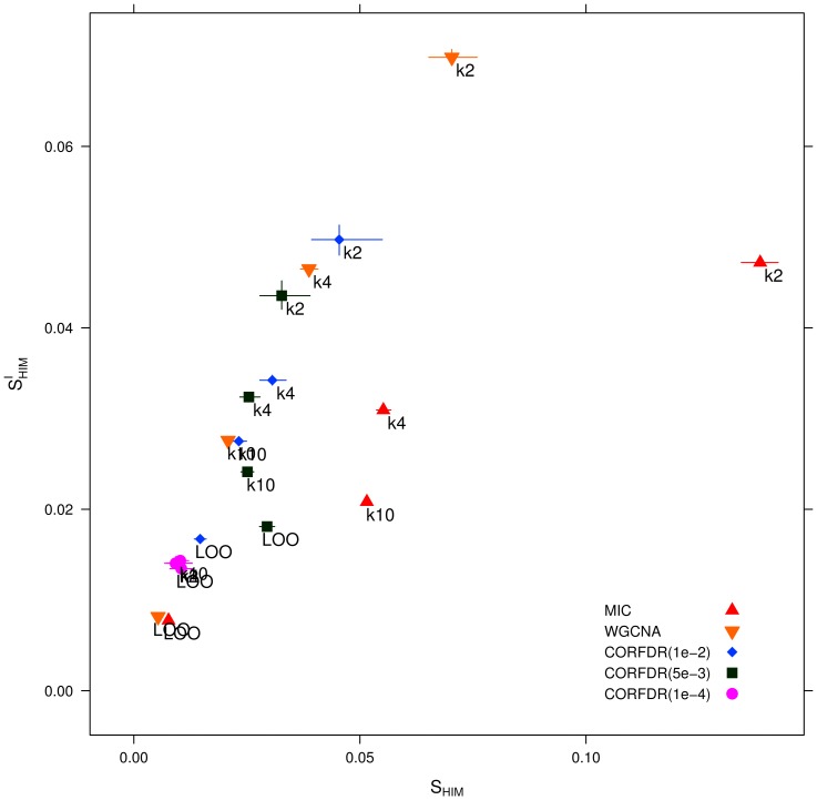
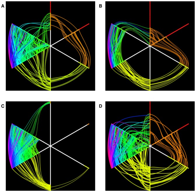
Each plot consists of six axes with lines connecting points lying on the axes themselves. The axis pointing upwards collects all the nodes with (unweighted) degree 0 or 1; , the next axis moving clockwise, is a copy of ; the following two axes include all nodes with degree 2, while on the remaining two axes lie all nodes with degree 3 or more. Different colors indicate different degree. Nodes on axes are ranked by degree. Lines between two consecutive axes show the network's edges and edge color is inherited by the node with smaller degree. Note the absence of links between nodes of degreee 1 and 2 in the FT case, and the smaller amount of connections between higher degree nodes in the MnT case with respect to the other three cases.

Figure 17. HCC-B dataset: mutual HIM distances for CLR inferred networks.

Comparison of the four networks Male Tumoral (MT), Male non Tumoral (MnT), Female Tumoral (FT) and Female non Tumoral (FnT) reconstructed from the whole corresponding subsets in Tab. (A) and in the derived 2D multidimensional scaling plot (B).

Figure 18. HCC-B dataset: and stability indicators of the four subgroups MT, MnT, FT, and FnT.

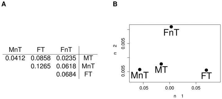
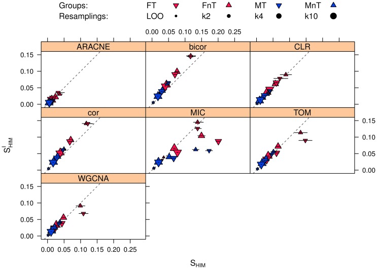
The networks are inferred with six different algorithms for different values of data subsampling. MT: Male Tumoral. MnT: Male non Tumoral. FT: Female Tumoral. FnT: Female non Tumoral. Confidence intervals are represented for each experiment. Points of increasing dimension are used to represent the diverse resampling schema: Leave One Out, -fold cross validation for set to 2 (), 4 () and 10 () respectively.