A network modeling approach for the spatial distribution and structure of bone mineral content

Abstract

This study aims to develop a spatial model of bone for quantitative assessments of bone mineral density and microarchitecture. A spatially structured network model for bone microarchitecture was systematically investigated. Bone mineral-forming foci were distributed radially according to the cumulative normal distribution, and Voronoi tessellation was used to obtain edges representing bone mineral lattice. Methods to simulate X-ray images were developed. The network model recapitulated key features of real bone and contained spongy interior regions resembling trabecular bone that transitioned seamlessly to densely mineralized, compact cortical bone-like microarchitecture. Model-simulated imaging profiles were similar to patients' X-ray images. The morphometric metrics were concordant with microcomputed tomography results for real bone. Simulations comparing normal and diseased bone of 20-30 to 70-80 year-olds demonstrated the method's effectiveness for modeling osteoporosis. The novel spatial model may be useful for pharmacodynamic simulations of bone drugs and for modeling imaging data in clinical trials.

Fig. 1

A simple two-dimensional schematic of the Voronoi tessellation modeling procedure used to creating a spatial model for bone. a An annular region representing bone. b The random distribution of Voronoi centers from a cumulative normal distribution function with μ = 0.3, σ = 0.02, and c ₀ = 1,500. c The result from Voronoi tessellation. d The Voronoi tessellation bounded by its outer boundary. e The result after the weights were assigned to the edges. f The weighted Voronoi tessellation after stochastic pruning

Fig. 2

A schematic of the procedures used to model arbitrary shapes. Each vertex of the Voronoi polyhedral on the circle (left) is mapped to the corresponding position on the arbitrary shape (right). The centroids of the circle and the arbitrary shape are denoted by C ₁ and C ₂, respectively. The points (R ₁, θ) and (R ₂, θ) are the radial coordinates on the boundary. The radial coordinates of the Voronoi vertex at (r ₁, θ) in the circle are mapped to the corresponding point (r ₂, θ) on the arbitrary shape using the constant of proportionality R ₂/R ₁

Fig. 3

The results from a three-dimensional implementation of the Voronoi tessellation modeling procedure. The six figures in the top two rows are the top-down views of the three-dimensional spatial structures obtained from steps shown in Fig. 1a–g. The lowest row shows the front views of the three-dimensional structures corresponding to Fig. 1b, e, and f. The outer surface was removed so that the interior can be seen h and i. The simulation parameters μ = 0.25, σ = 0.05, β = 0.5, and c ₀ = 3,000 were used

Fig. 4

Modeling bone images. a A section of the X-ray image of femur from a postmenopausal hip transplantation patient with BMD of 0.90 g/cm². b The distribution of image intensity across the radial section of bone shown as red line in a; also shows the normalized imaging intensity and the corresponding fit using the image modeling procedure. c, d The front and top view from a simulation with parameters μ = 0.25, σ = 0.05, β = 0.5, and c ₀ = 6000 containing 20 z slices, respectively. e A z stack obtained by simulating an X-ray image in transmission mode using the Radon transform on the model. f Obtained with a Gaussian filter to “smooth” the boundary of the z stack image of Fig. 4e. g Simply rotates Fig. 4e by a 3° angle so that it can be compared more effectively with the original X-ray image of Fig. 4a, which is tilted relative to the vertical

Fig. 5

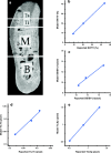
Modeling results for an irregular geometry. a An image of the mandible that was analyzed in detail by Moon et al (22). These authors derived quantitative morphometric measures in the alveolar region (marked with T _s and T _i), the basal bone superior to the mandibular canal (marked M) and the basal bone inferior to the mandibular canal (B). b–e Comparison of the results for bone volume fraction (BV/TV), bone surface density (BS/BV), trabecular thickness (Tb.Th), and trabecular separation (Tb.Sp), respectively, from the modeling to the measurements obtained by Moon et al (22). The simulation parameters were μ = 0.25, σ = 0.05, β = 1 and c ₀ = 4,000. The slopes for the best-fit lines in b–e were 0.924, 0.84, 1.02, and 1.21, respectively. The Pearson correlation coefficients were greater than 0.99 in each case

Fig. 6

Top views of simulations of normal and diseased bone. a, c, and e The bone mineral density values at the 95th percentile, 50th percentile (median), and 5th percentile for 20- to 30-year-old women, respectively. b, d, f Bone mineral density values at the 95th percentile, 50th percentile (median), and 5th percentile for 70- to 80-year-old women, respectively. The shape and dimensions were obtained from the report by Locke, and the mean bone mineral density values for these age groups were obtained from Looker et al (21). The 5th, 50th (median), and 95th percentiles for BMD of the 20- to 30-year-old groups were 0.870, 1.078, and 1.292 g/cm², respectively. The corresponding values for the 70- to 80-year-old groups were 0.731, 0.960, and 1.210 g/cm². The values of μ were 0.5 for a and b, and 0.25 for c–f. The values of σ were 0.05 for a–d and 0.025 for the e–f. The β values for a–f were 1,000, 1, 10, 1, 5, and 1, respectively. The value of c ₀ = 3,000 for a–f

References

1. Foundation IO. Facts and statistics: International Osteoporosis Foundation 2013. http://www.iofbonehealth.org/facts-statistics-category-14.
1. Johnell O, Kanis JA. An estimate of the worldwide prevalence and disability associated with osteoporotic fractures. Osteoporos Int J Established Result Cooperation Eur Found Osteoporos Nat Osteoporos Found USA. 2006;17(12):1726–33. doi: 10.1007/s00198-006-0172-4. - DOI - PubMed
1. Kanis JA. Assessment of osteoporosis at the primary health care level: report of a WHO Scientific Group. Sheffield, UK: World Health Organization; 2007.
1. Dennison E, Mohamed MA, Cooper C. Epidemiology of osteoporosis. Rheum Dis Clin N Am. 2006;32(4):617–29. doi: 10.1016/j.rdc.2006.08.003. - DOI - PubMed
1. Burge R, Dawson-Hughes B, Solomon DH, Wong JB, King A, Tosteson A. Incidence and economic burden of osteoporosis-related fractures in the United States, 2005–2025. J Bone Miner Res Off J Am Soc Bone Miner Res. 2007;22(3):465–75. doi: 10.1359/jbmr.061113. - DOI - PubMed
Publication types
LinkOut - more resources