Complex role of space in the crossing of fitness valleys by asexual populations

Abstract

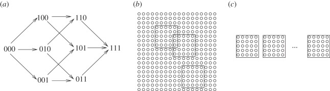
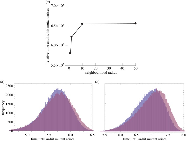
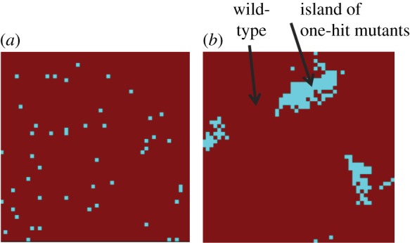
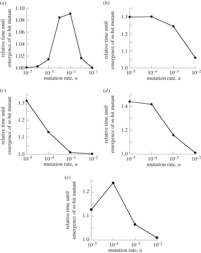
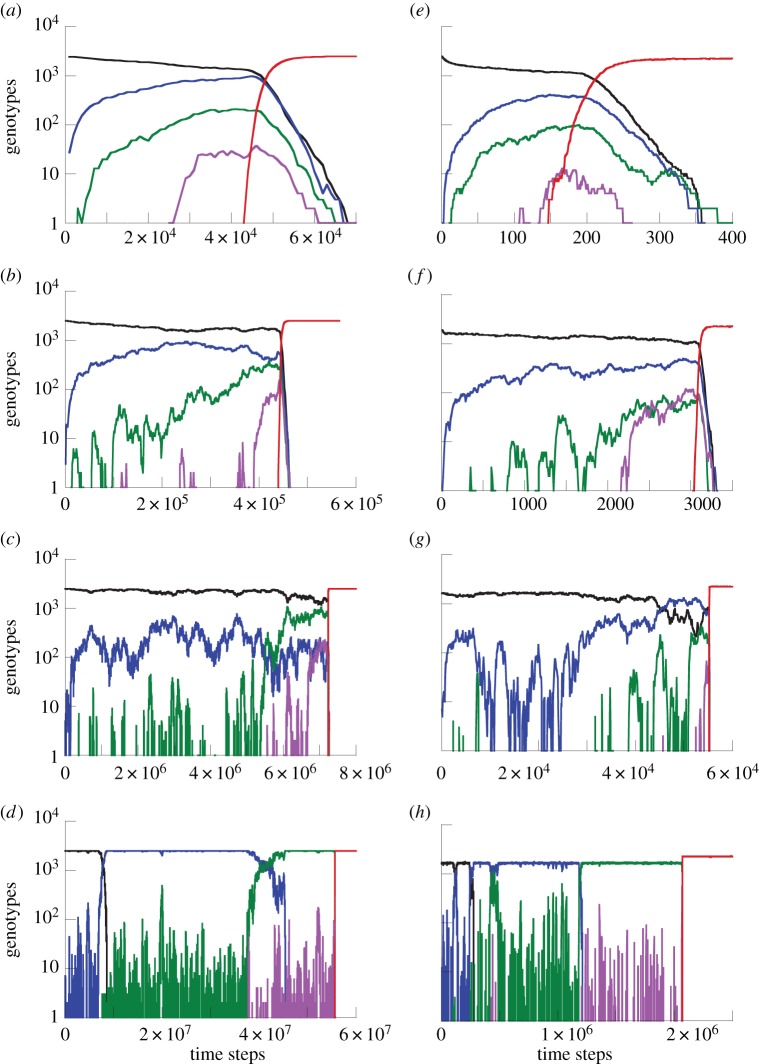
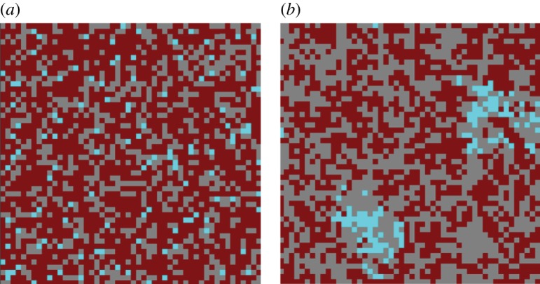
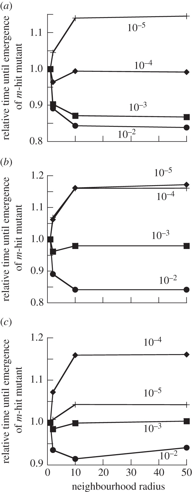
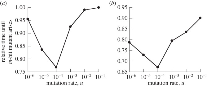
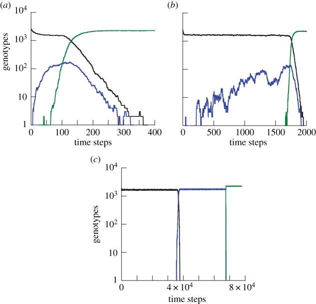
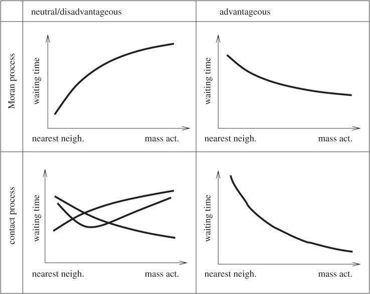
The evolution of complex traits requires the accumulation of multiple mutations, which can be disadvantageous, neutral or advantageous relative to the wild-type. We study two spatial (two-dimensional) models of fitness valley crossing (the constant-population Moran process and the non-constant-population contact process), varying the number of loci involved and the degree of mixing. We find that spatial interactions accelerate the crossing of fitness valleys in the Moran process in the context of neutral and disadvantageous intermediate mutants because of the formation of mutant islands that increase the lifespan of mutant lineages. By contrast, in the contact process, spatial structure can accelerate or delay the emergence of the complex trait, and there can even be an optimal degree of mixing that maximizes the rate of evolution. For advantageous intermediate mutants, spatial interactions always delay the evolution of complex traits, in both the Moran and contact processes. The role of the mutant islands here is the opposite: instead of protecting, they constrict the growth of mutants. We conclude that the laws of population growth can be crucial for the effect of spatial interactions on the rate of evolution, and we relate the two processes explored here to different biological situations.

Keywords: complex phenotype; mutations; sequential evolution; stochastic tunnelling.

Figure 1.

The simulation set-up. (a) The combinatorial mutation diagram for m = 3 sites. (b) The concept of neighbourhood, illustrated with the neighbourhoods of radius 2. (c) The patch model: the population is split into n patches. At each update, an individual is removed at random from a random patch, and is replaced by an offspring of another individual, chosen from the same patch according it its fitness.

Figure 2.

Effect of the neighbourhood radius on the time at which the m-hit mutant arises in the Moran process. (a) The average time of emergence for four neighbourhood radii: 1, 2, 10 and 50. Averages are based on at least 10⁵ iterations of the simulation. The chosen parameters were: grid size N = 50 × 50, m = 2, intermediate mutants were neutral, u = 10⁻⁴. (b) Histograms showing the distribution of outcomes, corresponding to the data presented in part (a). For the sake of simplicity, only two radii are compared: 1 and 50. (c) Same type of histogram, but with u = 10⁻⁵, showing a greater difference. (Online version in colour.)

Figure 3.

Spatial configuration of the Moran process for the case of (a) mass action and (b) a neighbourhood radius of 1. In the presence of spatial structure, islands of intermediate mutants are observed. The chosen parameters were: grid size = 50, m = 2, intermediate mutants were neutral, u = 10⁻⁴. (Online version in colour.)

Figure 4.

Time to emergence of m-hit mutant in the Moran process. Compared are mass action relative to extreme spatial restriction, where the neighbourhood radius is 1. The time to emergence for radius = 1 was set to unity, and the time observed for mass action was scaled accordingly. This number is plotted against the mutation rate, u. (a) m = 2, grid size N = 10 × 10, neutral intermediate mutants. (b) m = 2, N = 10 × 10, intermediate mutants have 10% fitness cost. (c) m = 2, N = 50 × 50, neutral intermediate mutants. (d) m = 2, N = 50 × 50, intermediate mutants have 10% fitness cost. (e) m = 4, N = 50 × 50, neutral intermediate mutants.

Figure 5.

Time-series simulation showing the evolutionary dynamics for (a–d) the Moran process and (e–h) the contact process, assuming m = 4, a 50 × 50 grid and neutral intermediate mutants. Wild-types are shown in black, intermediate one-, two- and three-hit mutants are shown in blue, green and pink, respectively. The advantageous four-hit mutant is shown in red. For the Moran process, the mutation rates were (a) u = 10⁻², (b) u = 10⁻³, (c) u = 10⁻⁴, (d) u = 10⁻⁵. For the contact process, L/D = 3, and (e) u = 10⁻², (f) u = 10⁻³, (g) u = 10⁻⁴ and (h) u = 10⁻⁵. The simulations were run under mass-action settings. (Online version in colour.)

Figure 6.

Spatial configuration of the contact process model for the case of (a) mass action and a neighbourhood radius of 1 (b). Grey depicts empty space. Wild-types are shown in dark (red), and one-hit mutants in light (cyan) colouring. In the presence of spatial structure, islands of intermediate mutants are observed. Individuals are not evenly distributed, but form macroscopic structures. The chosen parameters were: grid size 50 × 50, m = 2, intermediate mutants were neutral, u = 10⁻⁴, L/D = 3. (Online version in colour.)

Figure 7.

Numerically calculated densities of cells in the contact process, plotted as functions of the neighbourhood radius. We present the mean density (together with the empirical formula equation (3.2)), and the mean density of cells in a neighbourhood of non-empty spots (together with the empirical formula equation (3.3)). Also plotted is the pair approximation of the mean density. The parameters are N = 41 × 41, and L/D = 3. (Online version in colour.)

Figure 8.

Time to emergence of m-hit mutant in the contact process. Compared are neighbourhood radii of 1, 2, 10 and 50. The time to emergence for neighbourhood radius 1 was set to unity, and the waiting time observed for the other radii was scaled accordingly. Different curves are shown for different mutation rates u, as indicated in the plots. For all plots, L/D = 3. (a) m = 2, grid size is 50 × 50, neutral intermediate mutants. (b) m = 2, grid size is 50 × 50, intermediate mutants have 10% fitness cost. (c) m = 4, grid size is 50 × 50, neutral intermediate mutants.

Figure 9.

Time to emergence of m-hit mutant in (a) the Moran process and (b) the contact process, assuming that intermediate mutants are advantageous compared with the wild-type, and that the m-hit mutant is even more advantageous. Compared are mass action relative to extreme spatial restriction, where the neighbourhood radius is 1. The time to emergence for radius = 1 was set to unity, and the time observed for mass action was scaled accordingly. This number is plotted against the mutation rate, u. The other parameters were assigned the following values: m = 2, grid size N = 50 × 50, intermediate mutants have 10% fitness advantage. For (b) L/D = 3.

Figure 10.

Time-series simulations showing the evolutionary dynamics for the Moran process, assuming that intermediate mutants are advantageous and the m-hit mutant is even more advantageous. Plots are shown for three mutation rates: (a) 10⁻², (b) 10⁻⁴ and (c) 10⁻⁶. Wild-types are shown in black, intermediate mutants (i.e. one-hit mutants) in blue, and m-hit mutants in green. The simulations were done with m = 2, a 50 × 50 grid, and a 10% fitness advantage of intermediate mutants compared with wild-types. (Online version in colour.)

Figure 11.

A schematic summarizing the complex role of space in the generation time of m-hit mutants. The top row represents the Moran process, and the bottom row the contact process. The left column corresponds to neutral/disadvantageous intermediate mutants, and the right column to the advantageous intermediate mutants. In each graph, the horizontal axis represents the degree of mixing, from the nearest-neighbour model to the mass-action model. The curves show whether the waiting time increases or decreases (or is non-monotonic) as a function of the neighbourhood size. It also shows the relative size of the effect, when comparing the Moran process with the contact process.

References

1. Whitlock MC, Phillips PC, Moore FBG, Tonsor SJ. 1995. Multiple fitness peaks and epistasis. Annu. Rev. Ecol. Syst. 26, 601–629. (10.1146/annurev.es.26.110195.003125) - DOI
1. Weinreich DM, Chao L. 2005. Rapid evolutionary escape by large populations from local fitness peaks is likely in nature. Evolution 59, 1175–1182. - PubMed
1. Weissman DB, Desai MM, Fisher DS, Feldman MW. 2009. The rate at which asexual populations cross fitness valleys. Theor. Popul. Biol. 75, 286–300. (10.1016/j.tpb.2009.02.006) - DOI - PMC - PubMed
1. Hancock JF. 2003. RAS proteins: different signals from different locations. Nat. Rev. Mol. Cell Biol. 4, 373–385. (10.1038/nrm1105) - DOI - PubMed
1. Moolgavkar SH, Luebeck EG. 1992. Multistage carcinogenesis: population-based model for colon cancer. J. Natl Cancer Inst. 84, 610–618. (10.1093/jnci/84.8.610) - DOI - PubMed