A mesoscale connectome of the mouse brain

Abstract

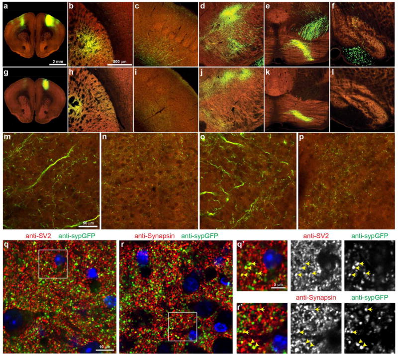
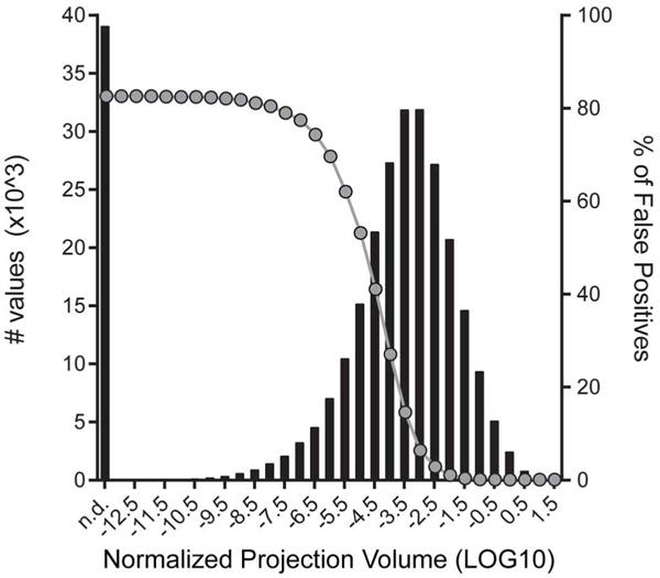
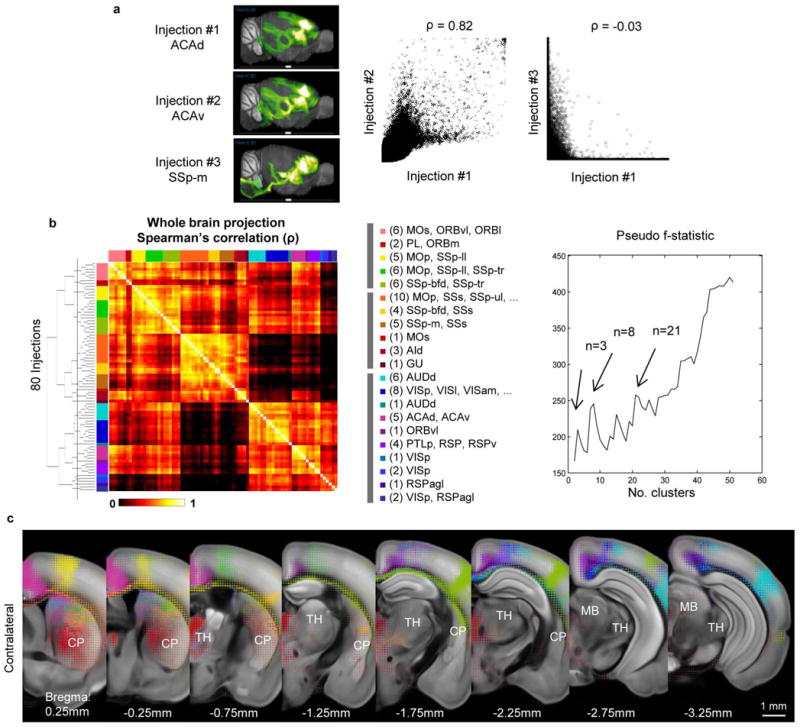
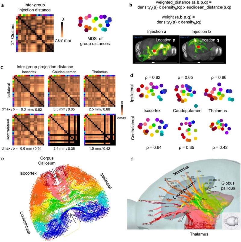
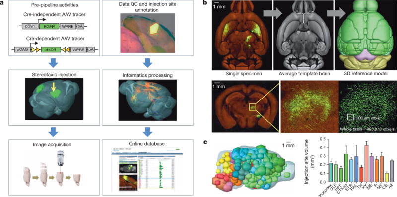
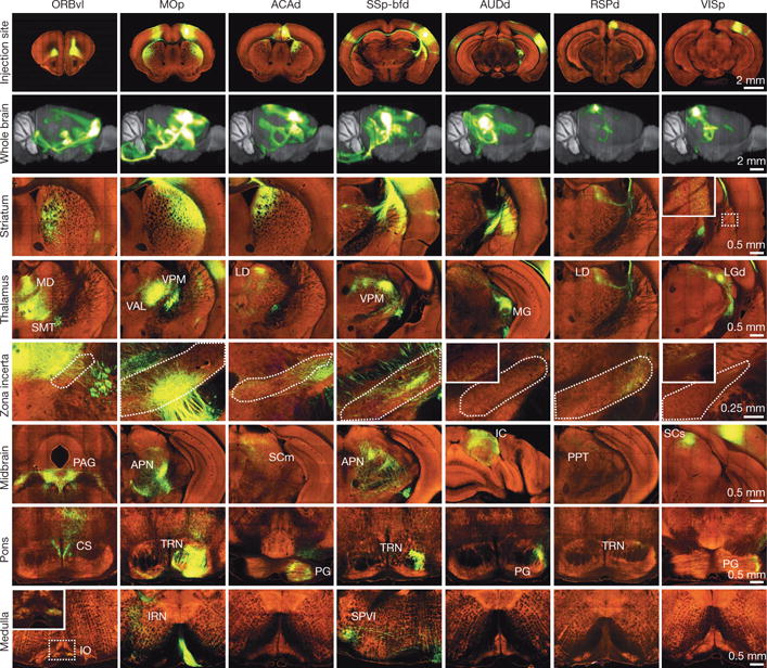
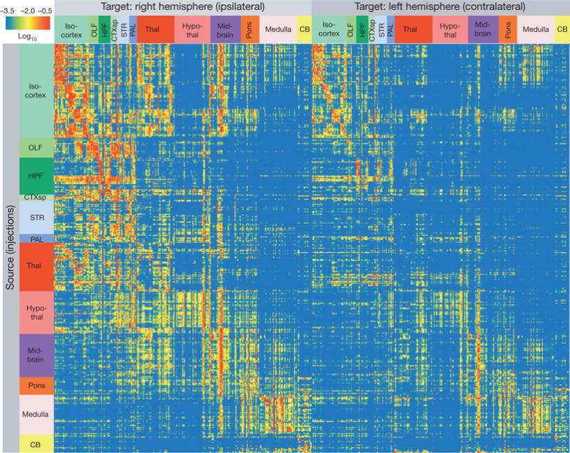
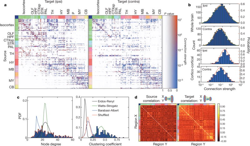
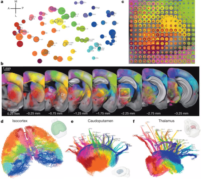
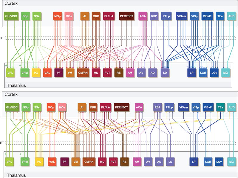
Comprehensive knowledge of the brain's wiring diagram is fundamental for understanding how the nervous system processes information at both local and global scales. However, with the singular exception of the C. elegans microscale connectome, there are no complete connectivity data sets in other species. Here we report a brain-wide, cellular-level, mesoscale connectome for the mouse. The Allen Mouse Brain Connectivity Atlas uses enhanced green fluorescent protein (EGFP)-expressing adeno-associated viral vectors to trace axonal projections from defined regions and cell types, and high-throughput serial two-photon tomography to image the EGFP-labelled axons throughout the brain. This systematic and standardized approach allows spatial registration of individual experiments into a common three dimensional (3D) reference space, resulting in a whole-brain connectivity matrix. A computational model yields insights into connectional strength distribution, symmetry and other network properties. Virtual tractography illustrates 3D topography among interconnected regions. Cortico-thalamic pathway analysis demonstrates segregation and integration of parallel pathways. The Allen Mouse Brain Connectivity Atlas is a freely available, foundational resource for structural and functional investigations into the neural circuits that support behavioural and cognitive processes in health and disease.

Extended Data Figure 1. AAV/BDA tracer comparison, using a primary motor cortex (MOp) injection as an example

The cortical and subcortical projections from MOp injection are labelled similarly with the AAV tracer (green) and conventional tracer BDA (red). a, Injection sites of AAV and BDA are mostly overlapping (yellow), with a blue DAPI counterstain. b, Confocal image taken from the box in a shows BDA tracer uptake in individual neurons at the injection site. b’, The same box in a shows AAV infection of individual neurons. b”, Overlay of b and b’ shows the presence of both tracers in the same region and their colocalization in some neurons (yellow). c–f, Examples of cortical projections in the contralateral primary motor cortex, ipsilateral primary somatosensory cortex, agranular insular area (dorsal part), and perirhinal cortex labelled with red, green, or yellow. g–n, Examples of subcortical projections in the ipsilateral ventral posterolateral nucleus of the thalamus and posterior nucleus of the thalamus, superior colliculus, pontine grey, caudate putamen, zona incerta and subthalamic nucleus, midbrain reticular nucleus, parabrachial nucleus, and contralateral bed nucleus of the anterior commissure. Scale bars are 1,000 μm (a); 100 μm in (b, b’ and b”); and 258 μm (c–n). Approximately 18 brain regions were selected throughout the brain to represent broad anatomical areas and diverse cell types (3 cortical and 15 subcortical structures). AAV and BDA were co-injected into each selected brain region in wild-type mice using a sequential injection method developed to target virtually the same anatomical region. For most cases, the anatomical area(s) of tracer uptake are well matched. We found the long-range projections from all studied regions with both tracers. Their patterns were similar between the two tracers in mostly overlapped injection cases. There were more retrogradely labelled neurons with BDA than AAV, although a few retrograde neurons were observed in all studied regions with both tracers. BDA was clearly uptaken by passing fibres in some injections but AAV was not.

Extended Data Figure 2. Consistency among individual STP tomography image sets

a, High-resolution images of 140 serial sections of a single brain are shown as an example (injection into the primary visual area). The injection site and major projection targets can be easily observed in this ‘contact-sheet’ view. b, Registration variability study. A set of ten 3D fiducial points of interest (POIs) were manually identified on the Nissl 3D reference space, the average template brain, and in 30 randomly selected individual image sets by three raters independently. The POIs were selected such that they span the brain and can be easily and repeatedly identified in 3D. Each POI (p) from each experiment was then projected into 3D reference space (p’) using the transform parameters computed by the Alignment module. Statistics were gathered on the target registration error between p’ and its ‘gold standard’ correspondence (computed as the mean of the labelling of 3 raters) in the Nissl (pNissl) and template (ptemplate) volumes. In summary, for all POIs in template space, the observed median variation in each direction are 28 μm for left-right, 35 μm for inferior-superior, and 49 μm for anterior-posterior. In Nissl space, these observed median variations are 42, 71 and 60 μm, respectively. The registration variations in different directions are shown here. For each POI, the green dot shows the position in template space (ptemplate) and the red dot shows the position in Nissl space (pNissl). The small yellow bar shows the median variation (among 30 image sets) away from ptemplate in each direction. POIs: AP: area postrema, midline; MM: medial mammillary nucleus, midline; cc1: corpus callosum, midline; cc2: corpus callosum, midline; acoL, acoR: anterior commisure, olfactory limb; arbL, arbR: arbor vitae; DGsgL, DGsgR: dentate gyrus, granule cell layer. c, Percent agreement between computationally assigned injection site voxels and manually assigned injection structures. Each histogram data point corresponds to a single injection, and 100% indicates that every injection site voxel was computationally assigned to a structure included on the manually annotated injection structures list. Voxels which were computationally assigned to fibre tracts or ventricles are excluded from the computation. Neither fibre tracts nor ventricles were incorporated into the manual annotation process; their exclusion allows for a more commensurate comparison.

Extended Data Figure 3. Distribution of injection sites across the brain

a, Locations of injection spheres within 12 major brain subdivisions are shown as a projection onto the mouse brain in sagittal views. n = 108 isocortex, 23 olfactory areas (OLF), 42 hippocampal formation (HPF), 8 cortical subplate (CTXsp), 38 striatum (STR), 9 pallidum (PAL), 57 thalamus (TH), 47 hypothalamus (HY), 50 midbrain (MB), 21 pons (P), 45 medulla (MY) and 21 cerebellum (CB). b, Frequency histogram for the injection site volumes of all 469 data sets is shown. c, The Allen Reference Ontology was collapsed into 295 non-overlapping, unique, anatomical structures for analyses, distributed across major brain subdivisions as shown (black bars). For most structures, a single injection was sufficient to infect the majority of neurons in that region. For larger structures (for example, primary motor cortex), multiple injections were made into several, spatially separate locations. The majority of these 295 regions have at least one injection targeted to that structure as either the primary or secondary injection site (white bars); only 18 structures are not covered at all (grey bars, for details see Supplementary Table 1). These missed structures (minimal to no infected cells in either the primary or secondary injection sites) were either very small (for example, nucleus y in the medulla), purposefully left out due to the presence of other injections under the same large parent structure (for example, four of the cerebellar cortex lobules), or technically challenging to reach via stereotaxic injection (for example, suprachiasmatic nucleus).

Extended Data Figure 4. Distribution of whole brain projections from different cortical source areas

Pie charts show the percentage of total projection volume across all voxels outside of the injection site distributed in the 12 major brain subdivisions from both hemispheres. Each pie chart represents the average of 4 to 27 cortical injections grouped by the broad regions listed. A pie chart key of the volume distribution (number of voxels per structure/total number of voxels per brain) of these 12 subdivisions is at the bottom right for comparison. The largest projection signal from each cortical injection is found within isocortex (range of 45.4–69.8% of projection signals depending on source region, with an average of 59% for all cortical injections), although the isocortex accounts for only 30.2% of total brain volume. Differences in the subcortical distribution of relative signal strength between cortical sources were also observed. For example, within the striatum (light blue), the percentage of total signal is low from auditory, retrosplenial and visual areas (6.2%, 3.4% and 7.6%, respectively), but much greater from frontal, motor, cingulate and somatosensory areas (16.5%, 27.7%, 20.3% and 17.6%, respectively).

Extended Data Figure 5. Variability of brain-wide projection signal strength

To examine animal-to-animal variability in projection patterns, 12 sources with two spatially overlapping injection experiments were identified from the full data set of tracer injections shown in Fig. 3. a, Rows show segmented projection volumes normalized to the injection volume (log₁₀-transformed) in the 295 ipsilateral target regions for each of 2 individual overlapping tracer injections per source region indicated (above and below solid black line). The colour map is as shown in Fig. 3. b, Maximal density projections of whole brain signals from each of the two spatially overlapping injection experiments per source region visibly demonstrate consistency of brain-wide connections. Scatter plots of all ipsilateral and contralateral target structure values above a minimum threshold in both members of the pair (log₁₀ = −3.5; non-blue values from a) show significant correlations between each pair of injections across a four orders of magnitude range of projection strengths. Values in the scatter plots are Pearson’s correlation coefficients (r). Note that in some cases (for example, PTLp) axon pathways appear to be labelled in only one of the pair. This could be due to random differences in the proportion of corticospinal projecting neurons labelled in a particular injection within the same source area. Signal in large annotated white matter tracts are computationally removed from the connectivity matrix, and thus not included in the scatter plots. c, Detected fluorescent signals from each of two injections into the same location of primary somatosensory cortex registered and overlaid with the average template brain (grey). Lower 2 rows, 2D raw images from each injection experiment at different anterior-posterior levels. The centres of these injection sites are in the far left panel and their major targets are in the right panels. See Supplementary Table 1 for the corresponding full name and acronym for each region.

Extended Data Figure 6. Cytoplasmic EGFP and synaptophysin-EGFP AAV tracer comparison, using primary motor cortex (MOp) injections as an example

a–f, Two-photon images showing an example of the labelling obtained using the Phase I virus for whole-brain projection mapping, which consists of a human Synapsin I promoter driving expression of EGFP. g–l, To compare cytoplasmic labelling of projections and identification of terminal regions with a presynaptic reporter virus, we made a construct with the same hSynapsin promoter driving expression of a triple reporter cassette (AAV2/1.pSynI.nls-hrGFP-T2A-tagRFP-T2A-sypGFP.WPRE.bGH): a nuclear localization signal attached to humanized Renilla GFP (nls-hrGFP), a T2A sequence followed by cytoplasmic tagRFP, a second T2A sequence, and the synaptophysin-EGFP fusion (sypGFP). Owing to the two-photon imaging wavelength used (925 nm), the tagRFP (red) signal is weak to non-existent in these images. a, g, An image at the centre of the infected area after injection into the same region of MOp with the Phase I cytoplasmic viral tracer (a) and the nuclear and synaptic reporter viral tracer (g). Examples of viral labelling in the caudoputamen (b, h), somatosensory cortex (c, i), thalamus (d, j), pontine grey (e, k) and inferior olivary complex in the medulla (f, l) are shown for both tracers. The cytoplasmic viral tracer labels axons, revealing dense branching patterns in presumed terminal zones. The presynaptic reporter virus predominantly shows a punctate pattern of labelling consistent with presynaptic protein expression patterns, and indicative of terminal zones. Punctate or diffuse labelling was observed with the synaptic reporter virus in nearly all MOp target regions manually and computationally identified using the cytoplasmic reporter, including those with both large and small signals. Fluorescent signal originating in fibres outside of large white matter tracts are included in the signal quantification and matrix shown in Fig. 3, but signals from these large annotated fibre tracts are computationally removed. m–p, High-resolution images of terminal zones in the somatosensory cortex (m) and thalamus (o) identified using the cytoplasmic viral tracer show axon ramification and punctate structures consistent with bouton labelling, similar to the synaptic reporter in the corresponding regions (n, p). q–r’, To validate the presynaptic expression of the sypGFP fusion protein, sections including and adjacent to the thalamic region shown in j were collected after two-photon imaging and immunostained with antibodies against GFP (chicken polyclonal 1:500, Aves Labs, Inc. #GFP-1020) and synapsin I (rabbit polyclonal, 1:200, Millipore, #AB1543P) or GFP (rabbit polyclonal, Life Technologies, #A-11122) and SV2 (mouse monoclonal, DSHB, SV2-supernatant) presynaptic proteins. q, r, Confocal images at a single plane show punctate labelling indicative of presynaptic boutons for both sypGFP and synapsin or SV2. Many puncta were colocalized (yellow arrows show select examples in q’ and r’), although quantification was not reliable due to the very high density of presynaptic labelling by anti-Synapsin and anti-SV2.

Extended Data Figure 7. Distribution of log₁₀-transformed normalized projection volumes from the entire matrix presented in Fig. 3

The values (left-hand y axis, black bars) were number of target regions and derived from Supplementary Table 2. The entire range of the normalized projection volumes in this matrix was between log₁₀ = −14 and log₁₀ = 1.5, and it peaked between log₁₀ = −3.5 and log₁₀ = −3.0. A manual analysis of true positive and true negative signals from 20 randomly chosen injection experiments, representing the range of injection sizes, was used to estimate the false positive rate at different threshold levels, shown on the right-hand y axis (grey circles). True positive values predominantly fall within the range of log₁₀ = −4 to 1.5. For example, at a threshold of log₁₀ = −4, the false positive rate was 27%, dropping to 14.5% at log₁₀ = −3.5. False positives were almost exclusively due to small segmentation artefacts in areas without actual fluorescently labelled axon fibres.

Extended Data Figure 8. Cortical domains identified by clustering analysis of projection patterns

Eighty injections were used in the analysis for which the injection site is strictly within the isocortex and injection volume >0.07 mm³. a, Scatter plot of the voxel densities (excluding injection sites) of the whole brains from two nearby anterior cingulate injections (ACAd and ACAv) shows a strong correlation between the two (Spearman’s ρ = 0.82), whereas that of two distant injections (ACAd and SSp-m) shows little correlation (ρ = −0.03). b, Hierarchical clustering of the projection pattern based on Spearman’s rank correlation coefficient of voxel density over the entire brain. The pseudo-F statistics measures the coherence of clusters and is the ratio of mean sum of squares between groups to the mean sum of squares within group. Peaks in the pseudo-F statistics (for example, at n = 3, 8 and 21 clusters) are indicators of greater cluster separation. For n = 21 clusters, a systematic colour-code is given to each cluster to provide a visual guide to their cortical location (Fig. 5a), the numbers in parentheses indicate the number of injections in each group. c, Voxel densities from the 21 selected injections from Fig. 5a are overlaid as ‘dotograms’ at 8 coronal levels for the contralateral hemisphere.

Extended Data Figure 9. Topography of cortico-striatal and cortico-thalamic projections

Average inter-group distance was used to quantify the degree of which inter-group spatial relationship within the cortex is preserved in target domains. a, Inter-group injection distances were obtained by computing the 3D Euclidean distances between injection site voxels of two experiments, one from each group, and then averaging over all injection pairs. For visualization, the distances are embedded into a 2D plane using multidimensional scaling to create a group-level injection flat-map. b, Inter-group projection distances were obtained by computing the 3D Euclidean distance between a pair of voxels in a target domain weighted by the product of voxel density of two injections, one from each group. The distances are then averaged over all voxel pairs in the target domain and injection pairs between groups. c, Inter-group projection distance matrices for each target domain visualized as false-coloured heatmaps. The black columns and rows in contralateral caudoputamen and thalamus are due to four missing structures. d, Inter-group projection distances are embedded into a 2D plane using multidimensional scaling to visualize the spatial relationship between groups. e, 3D tractography paths from decimated (every other indices in each dimension) voxels in both cortical hemispheres. Voxels belonging to the medial cortical groups have been omitted to reveal a reconstructed corpus callosum showing parallel crossings with a conserved spatial configuration. f, A top-down view of 3D tractography paths into the ipsilateral thalamus for all voxels excluding the RSP/VIS groups showing axonal projections passing through fibre tracts in the striatum, narrowing through the globus pallidus, before spreading throughout the thalamus.

Extended Data Figure 10. A matrix of major connections between functionally distinct cortical regions and thalamic nuclei, corresponding to Fig. 6

Upper and lower panels show projections from cortex (source) to thalamus (target) or from thalamus (source) to cortex (target), respectively (ipsilateral projections only). The label ‘pc’ indicates that cortico-thalamic and thalamo-cortical projections in the gustatory/visceral pathway are between GU/VISC cortical areas and VPMpc/VPLpc nuclei. The number of pluses denotes relative connectivity strength and corresponds to the thickness of arrows in Fig. 6. All the connections described here were found in our data set. Connections labelled in red are previously known, whereas those labelled in black are not previously described in the rodent literature to our knowledge. There are also cases in which a connection was described in the literature but is excluded here because we could not find solid evidence in our data set to support it. All references that we have used to compare with our data are listed^,,–. Specifically, the cortico-thalamic system can be divided into six functional pathways: visual, somatosensory, auditory, motor, limbic and prefrontal. The visual pathway is composed of primary and associational visual cortical areas (VISp, VISam, VISal/l, and TEa) and thalamic nuclei LGd, LGv, and LP^,,, with LGd and VISp playing primary roles in processing incoming visual sensory information, visual associational areas involved in higher-order information processing and LP potentially modulating the function of all visual cortical areas (thus similar to the pulvinar in primates). LGv does not project back to cortex. Similarly, the somatosensory pathway is composed of primary and secondary somatosensory cortical areas (SSp and SSs) and thalamic nuclei VPM, VPL and PO^,, with SSp and VPM/VPL playing primary roles in processing incoming somatosensory information, SSs in higher-order information processing and PO modulating the function of all somatosensory cortical areas. The gustatory and visceral pathway (involving GU/VISC cortical areas and VPMpc/VPLpc nuclei)^, and the auditory pathway (involving primary and secondary AUD areas and different MG nuclei)^, also have similar organizations, although our current data do not have sufficient resolution to resolve fine details. The motor pathway is composed of primary and secondary motor cortical areas (MOp and MOs) and the VAL nucleus^,. The limbic pathway (which is closely integrated with the hippocampal formation system not discussed here) is composed of the retrosplenial (RSP) and anterior cingulate (ACA) cortical areas and thalamic nuclei AV, AD and LD^,. The prefrontal pathway, which is considered to play major roles in cognitive and executive functions, is composed of the medial, orbital and lateral prefrontal cortical areas (including PL, ILA, ORB and AI) and many of the medial, midline, and intralaminar nuclei of the thalamus (including MD, VM, AM, PVT, CM, RH, RE and PF). The reticular nucleus (RT) is unique in that it is a relay nucleus for all these pathways, receiving collaterals from both cortico-thalamic and thalamo-cortical projections although itself only projecting within the thalamus. Between these pathways, we have observed cross-talks, mediated by specific associational cortical areas and thalamic nuclei that may be considered to play integrative functions. For example, the anterior cingulate cortex (ACA) appears to bridge the prefrontal and the limbic pathways, interconnecting extensively with both. The posterior parietal cortex (PTLp) and the LD nucleus may relay information between the visual and the limbic pathways. PTLp, while hardly receiving any inputs from the thalamus, projects strongly to both LP and LD. On the other hand, LD, while projecting quite exclusively to the limbic cortical areas, receives strong projections from all visual cortical areas. There is also extensive cross-talk between the motor pathway and the prefrontal pathway, with both MOp and MOs receiving strong inputs from VM and sending strong projections to MD, and additionally with MOs projecting widely into many medial, midline and intralaminar nuclei. Finally, the thalamic nuclei PO, VM, CM, RH and RE all send out widely distributed, albeit weak, projections to many cortical areas in different pathways, thus potentially capable of modulating activities in large cortical fields.

Figure 1. Creation of the Connectivity Atlas

a, The data generation and processing pipeline. QC, quality control. b, The two main steps of informatics data processing: registration of each image series to a 3D template (upper panels) and segmentation of fluorescent signal from background (lower panels). c, Distribution of injection sites across the brain. The volume of the injection was calculated and represented as a sphere. Locations of all these injection spheres are superimposed together (left panel). Mean injection volumes (± s.e.m.) across major brain subdivisions are shown (right panel, see Extended Data Fig. 3).

Figure 2. Whole brain projection patterns from seven representative cortical regions

One coronal section at the centre of each injection site is shown in the top row (see Supplementary Table 1 for the full name of each region). In the second row, 3D thumbnails of signal density projected onto a sagittal view of the brain reveal differences in brain-wide projection patterns. The bottom 6 rows show examples of EGFP-labelled axons in representative subcortical regions.

Figure 3. Adult mouse brain connectivity matrix

Each row shows the quantitative projection signals from one of the 469 injected brains to each of the 295 non-overlapping target regions (in columns) in the right (ipsilateral) and left (contralateral) hemispheres. Both source and target regions are displayed in ontological order. The colour map indicates log₁₀-transformed projection strength (raw values in Supplementary Table 2). All values less than 10^−3.5 are shown as blue to minimize false positives due to minor tissue and segmentation artefacts and all values greater than 10^−0.5 are shown as red to reduce the dominant effect of projection signals in certain disproportionately large regions (for example, striatum).

Figure 4. A computational model of inter-regional connection strengths

a, The inter-region connectivity matrix, with connection strengths represented in colours and statistical confidence depicted as an overlaid opacity. Note that in this matrix, the sources (rows) are regions, whereas for the matrix of Fig. 3, the sources are injection sites. b, Both whole-brain and cortico-cortical connections can be fit by one-component lognormal distributions (red lines). However, the log distributions of whole-brain connection strengths are best fit by a two-component Gaussian mixture model (green lines). c, Node degree and clustering coefficient distributions for a binarized version of the linear model network, compared against Erdos-Renyi, Watts-Strogatz and Barabasi-Albert networks with matched graph statistics. d, Comparison of the correlation coefficients of normalized connection density between areas, defined as the common source for projections to other regions (left) and as the common target of projections from other regions (right).

Figure 5. Topography of cortico-striatal and cortico-thalamic projections

a, Cortical domains in the cortex flat-map. Each circle represents one of 80 cortical injection experiments, whose location is obtained via multidimensional scaling from 3D to allow visualization of all the sites in one 2D plane. The size of the circle is proportional to the injection volume. Clustered groups from Extended Data Fig. 8b are systematically colour-coded. The selected injections for b are marked with a black outline. b, For co-visualization, voxel densities from the 21 selected injections from a are overlaid as ‘dotograms’ at 8 coronal levels for ipsilateral hemisphere. For the dotogram, one circle, whose size is proportional to the projection strength, is drawn for each injection in each voxel; the circles are sorted so that the largest is at the back and the smallest at the front, and are partially offset as a spiral. c, Enlarged view of the dotogram from the area outlined by a white box in b. d, 3D tractography paths in both cortical hemispheres. e, A medial view of 3D tractography paths into the ipsilateral caudoputamen. Voxel starting points are represented as filled circles and injection site end points as open circles. f, A top-down view of 3D tractography paths into the ipsilateral thalamus.

Figure 6. A wiring diagram of connections between major cortical regions and thalamic nuclei

Upper and lower panels show projections from cortex to thalamus or from thalamus to cortex, respectively (ipsilateral projections only). Colour coding of different cortical regions and their corresponding thalamic nuclei is similar to the flat-map cortex in Fig. 5a. Thickness of the arrows indicates projection strength, which is shown in three levels as in Extended Data Fig. 10 and corresponds roughly to the red, orange and yellow colours in the raw connectivity matrix (Fig. 3). LGv and PF do not have significant projections to cortex. The reticular nucleus of the thalamus (RT) (the dashed box) is placed in between cortex and thalamus to illustrate its special role as a relay nucleus which all cortico-thalamic and thalamo-cortical projections pass through and make collateral projections into. The asterisks indicate that cortico-thalamic and thalamo-cortical projections in the gustatory/visceral pathway are between GU/VISC cortical areas and VPMpc/VPLpc nuclei (instead of VPM/VPL). See Supplementary Table 1 for the full name of each region.

References

1. Swanson LW. Brain Architecture: Understanding the Basic Plan. Vol. 331. Oxford Univ. Press; 2012.
1. Seung S. Connectome: How The Brain’s Wiring Makes Us Who We Are. Vol. 359. Houghton Mifflin Harcourt; 2012.
1. Sporns O. Networks of the Brain. Vol. 412. The MIT Press; 2011.
1. White JG, Southgate E, Thomson JN, Brenner S. The structure of the nervous system of the nematode Caenorhabditis elegans. Phil Trans R Soc Lond B. 1986;314:1–340. - PubMed
1. Felleman DJ, Van Essen DC. Distributed hierarchical processing in the primate cerebral cortex. Cereb Cortex. 1991;1:1–47. - PubMed
Publication types