Variable timing of synaptic transmission in cerebellar unipolar brush cells

Abstract

The cerebellum ensures the smooth execution of movements, a task that requires accurate neural signaling on multiple time scales. Computational models of cerebellar timing mechanisms have suggested that temporal information in cerebellum-dependent behavioral tasks is in part computed locally in the cerebellar cortex. These models rely on the local generation of delayed signals spanning hundreds of milliseconds, yet the underlying neural mechanism remains elusive. Here we show that a granular layer interneuron, called the unipolar brush cell, is well suited to represent time intervals in a robust way in the cerebellar cortex. Unipolar brush cells exhibited delayed increases in excitatory synaptic input in response to presynaptic stimulation in mouse cerebellar slices. Depending on the frequency of stimulation, delays extended from zero up to hundreds of milliseconds. Such controllable protraction of delayed currents was the result of an unusual mode of synaptic integration, which was well described by a model of steady-state AMPA receptor activation. This functionality extends the capabilities of the cerebellum for adaptive control of behavior by facilitating appropriate output in a broad temporal window.

Keywords: neural timing; spreading diversity.

Fig. 1.

Properties of the EPSC. (A) Epifluorescence image of a UBC filled through the patch pipette with a fluorescent dye. (B) Example recordings of responses to a single presynaptic stimulus from two different UBCs. (Insets) enlargement of the fast EPSC. (Vertical scale bars, 50 pA.) Red markers indicate the time of stimulation; artifacts were removed for clarity. Traces are averages of 10 sweeps. 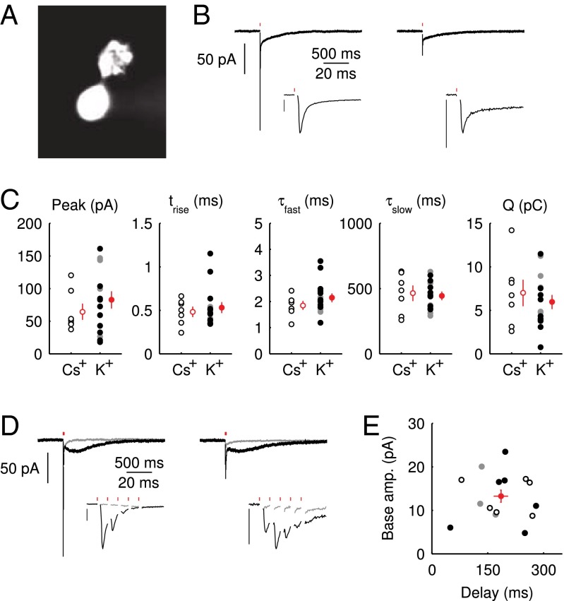(C) Summary of EPSC properties from 22 UBCs, Left to Right: peak amplitude, rise time , decay time constant of the fast EPSC , decay time constant of the slow tail , and total charge transferred . Filled dots, K⁺-based internal. Open dots, Cs⁺-based internal. All data were taken at , except for the filled gray dots, which were taken at (n = 2) or (n = 3). Average and SEM are shown in red. (D) Response to burst stimulation of the same cells as in A, averages of five sweeps. (E) Amplitude vs. delay of the maximal slow EPSC from 15 UBCs.

Fig. 2.

Steady-state EPSCs. (A) Examples of steady-state EPSCs, derived from regular stimulation protocols at increasing frequencies. The transparent red lines indicate the baseline slope, which is the slope of the EPSC just before stimulation. (B–D) Summary of steady-state EPSC peaks, baseline amplitudes, and baseline slopes, respectively, as a function of stimulation frequency for eight UBCs. As sample frequencies varied between cells, averages and SEM (red) were obtained by interpolation.

Fig. 3.

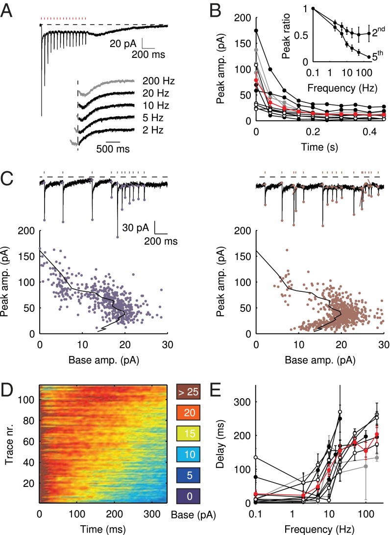
Delayed EPSC generation. (A) UBC response to a regular 20-Hz stimulus train. (Inset) Example traces of slow waves following regular stimulation at different frequencies. The 200-Hz curve was redrawn in gray beneath each trace for comparison. The vertical dotted line was drawn 20 ms after the final stimulus in the train. (B) Adaptation of EPSC peaks during 20-Hz stimulus trains ; average and SEM are shown in red. (Inset) EPSC peak ratio (relative to the first EPSC) of the second and fifth peaks in a train, as a function of train stimulus frequency. (C) Example traces of responses to irregular stimulation (single sweep, 90 s) at average frequencies 5 (Upper Left, blue) and 10 Hz (Upper Right, red). Stimulation times, peaks of the fast EPSCs, and baseline currents before stimulations are indicated by markers. In the lower panels, EPSC peaks are plotted vs. the corresponding baseline currents for 5 (Lower Left, blue dots) and 10 Hz (Lower Right, red dots). Steady-state values derived from Fig. 2 are replotted here for this particular cell (black curve). (D) Heatmap of stacked traces of slow synaptic current during irregular stimulation of the cell in A. Traces with ISIs ≥ 350 ms were selected and sorted according to the value of baseline current at time 350 ms. (E) Latency of the maximal slow EPSC following regular stimulation, as a function of frequency for 11 UBCs. Individual curves resulted from at least five repetitions, and error bars indicate SD. The average curve is plotted in red, with error bars indicating SEM.

Fig. 4.

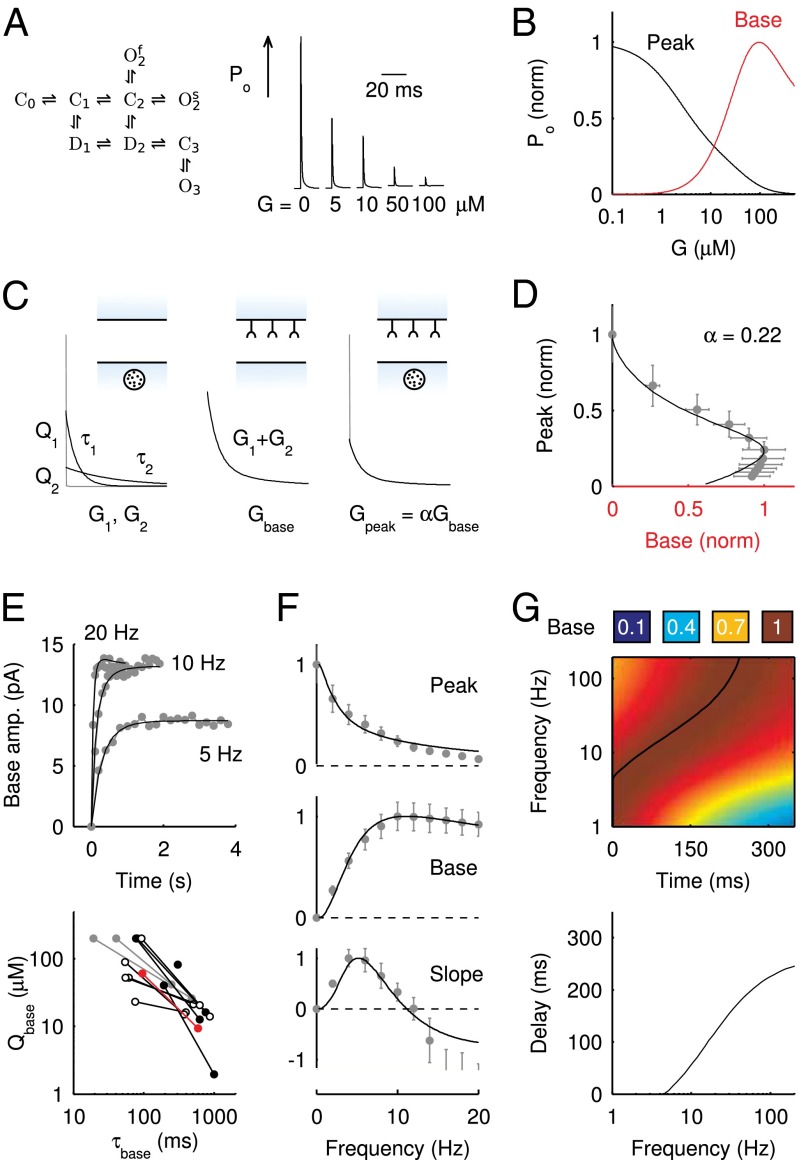
AMPAR model simulations. (A) Schematic representation of the AMPAR model from Raman and Trussell (2). Traces are simulation results of total (summed) receptor open probability P_o in response to a 4-mM pulse of glutamate for five values of the ambient glutamate concentration G. (B) Peak P_o in response to a brief 4-mM glutamate pulse (black trace) as a function of G. The steady-state P_o as a function of G is plotted in red. (C) Glutamate release and decay model. The background glutamate concentration G was modeled as an instantaneously released quantity, which decayed biexponentially to zero (black). The gray curves represent the fast glutamate peak (truncated) underlying the fast EPSC. Further details are described in the main text. (D) as a function of (black curve). The steady-state AMPAR model was fitted to experimental steady-state data (gray) with fit parameter α. (E) Results of fitting the biexponential glutamate decay model to EPSC base amplitudes obtained from regular stimulation experiments (Upper). Each fit was characterized by a pair of release amplitudes and decay time constants ; results are shown in the bottom panel for 11 UBCs. (F) Model fit to steady-state data of Fig. 2. Fit results are shown in red in E. (G) (Upper) as a function of time following 10 regular stimuli at varying stimulation frequency. The black curve denotes the time of maximal . (Lower) Delay of the maximal as a function of stimulation frequency for 10 stimuli.

Fig. 5.

Modulation of action potential generation. (A) Examples of modulation of action potential firing in response to direct somatic injection of sinusoidal currents at 1 and 2 Hz. (Top) Injected current. (Middle) Recorded voltage. (Bottom) Average instantaneous firing rate from 20 (1 Hz) and 40 (2 Hz) sweeps. (B) Gain and phase of the input-output transformation as a function of sinusoidal frequency for a total of 21 UBCs. The trace corresponding to the example cell in A is shown in black; average and SEM are shown in red.