Navigational strategies underlying phototaxis in larval zebrafish

Abstract

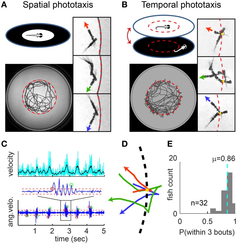
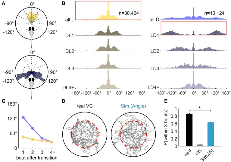
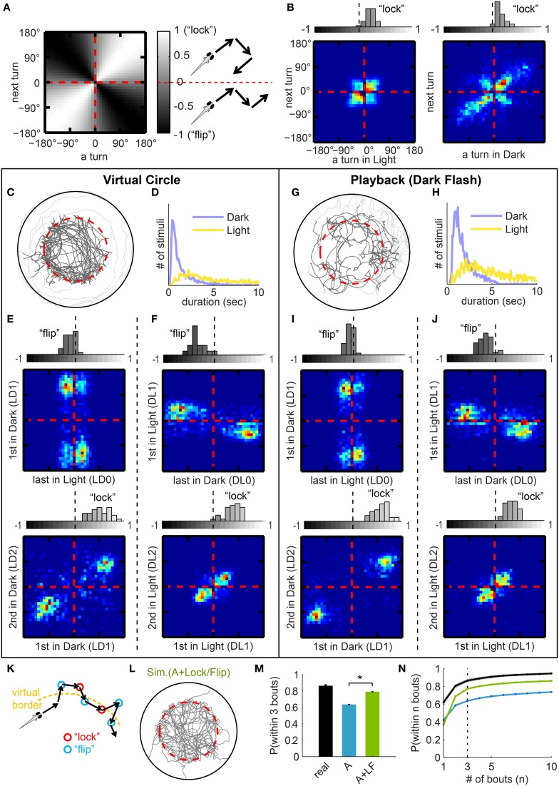
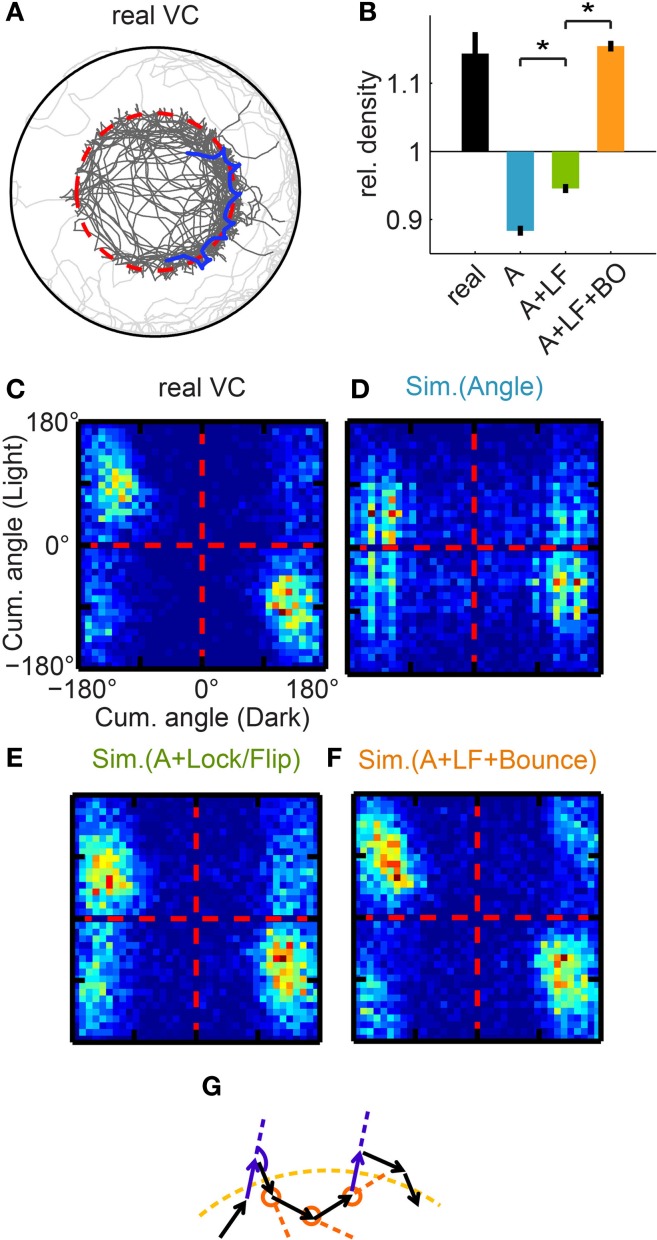
Understanding how the brain transforms sensory input into complex behavior is a fundamental question in systems neuroscience. Using larval zebrafish, we study the temporal component of phototaxis, which is defined as orientation decisions based on comparisons of light intensity at successive moments in time. We developed a novel "Virtual Circle" assay where whole-field illumination is abruptly turned off when the fish swims out of a virtually defined circular border, and turned on again when it returns into the circle. The animal receives no direct spatial cues and experiences only whole-field temporal light changes. Remarkably, the fish spends most of its time within the invisible virtual border. Behavioral analyses of swim bouts in relation to light transitions were used to develop four discrete temporal algorithms that transform the binary visual input (uniform light/uniform darkness) into the observed spatial behavior. In these algorithms, the turning angle is dependent on the behavioral history immediately preceding individual turning events. Computer simulations show that the algorithms recapture most of the swim statistics of real fish. We discovered that turning properties in larval zebrafish are distinctly modulated by temporal step functions in light intensity in combination with the specific motor history preceding these turns. Several aspects of the behavior suggest memory usage of up to 10 swim bouts (~10 sec). Thus, we show that a complex behavior like spatial navigation can emerge from a small number of relatively simple behavioral algorithms.

Keywords: behavior; modeling; navigation; phototaxis; zebrafish.

Figure 1

Spatial vs. temporal phototaxis. (A) Larval zebrafish prefer light over darkness in the spatial comparison assay. Upper left: a diffusive (scattering) white screen surrounded by an opaque black ring is placed beneath the arena (a transparent dish) and illuminated from below. Lower left: the full trajectory of a fish over a session of 8 min. Right panels: close-up views of trajectory segments close to the border. Three example segments are shown (rotated into the same orientation), with swim direction indicated by the red, green, and blue arrowheads; circular border indicated by the dashed red line. Note that the fish does not cross the border. (B) Temporal comparison assay, i.e., the Virtual Circle (VC) assay. The uniform illumination is turned off when the fish exits the virtual circle (dashed red circle, invisible to fish), and turned on again when the fish returns. Close-up view as in (A), additionally with yellow dots marking the point where the fish exits the virtual circle. (C) Larval zebrafish swim in distinct bouts. Upper panel: velocity of the fish over time. Lower panel: bouts are determined by thresholding the angular velocity (i.e., per-frame change of heading angle); red/green circles mark the start/end of bouts, dashed red lines mark the thresholds. (D) Trajectory segments close to the virtual border are extracted from the VC assay, with the point where fish exits the border aligned to the yellow dot. Three example segments are shown in red, green and blue, with swim direction indicated by arrowhead. (E) The probability of each fish returning to light within 3 bouts of exiting the virtual circle, summarized as a histogram for all 32 fish. Dashed cyan line indicates population mean.

Figure 2

Turning-angle distributions in the light, in the dark, and at transitions. (A) Turning-angle distributions from an example fish. Upper panel: all turns in light. Lower panel: the first turn after the Light-to-Dark transition (LD1) is usually a large angle turn. (B) Turning-angle distributions from all 32 fish, for bouts in light (left panel) and in dark (right panel). The top two histograms summarize all turns made in light (left) and in dark (right), respectively. “DLn”: the n-th turn after a Dark-to-Light transition. DL4+: all subsequent turns in the dark. “LD”: respective turns in response to a Light-to-Dark transition. Histograms framed in red correspond to the single-fish polar plots in (A). (C) Mean turning angle—after excluding center peaks—of the n-th turn after transitions, extracted from (B). (D) Example trajectories of real and simulated sessions (using Algorithm I [Angle], i.e., turning-angle distributions in B) for the Virtual Circle assay. Fish trajectory is shown in gray; dashed red circle marks the virtual border. Traces after the fish reached the edge of the arena and before it returned to within the virtual borders are not shown (see Materials and Methods). (E) The average probability of returning to light within 3 bouts of exiting the virtual circle (similar to Figure 1E), compared between real fish (n = 32), a control simulation (“ctrl,” n = 100) that implements a generic turning-angle distribution pooled from all turns, and the simulation (n = 100). [Mean ± s.e.m, ^*p < 0.001 (paired t-test) for all pairs].

Figure 3

Turning modulation around light transitions. (A) Value map of “lock-index” for correlation matrices (B,E,F,I,J). For a pair of consecutive turns, “locked” turns (2 turns in the same direction) populate the white diagonal (correlation), and “flipped” turns (2 turns in opposite directions) the black diagonal (anti-correlation). The lock-index ranges from −1 to 1, −1 being “flipped” (with identical turning magnitudes) and 1 being “locked.” (B) Correlation matrices for consecutive turns, data pooled from all 32 fish. Left panel: all pairs of consecutive turns in light. Most are small angle turns, and fish have a small bias for “lock.” Right panel: all pairs of consecutive turns in dark. Most large angle turns are “locked” in the same direction. Above each matrix: corresponding histograms of average lock-indices for each fish, calculated with (A). (C) Sample trajectory of Virtual Circle experiment. Traces after the fish reached the edge of the arena and before it returned to within the virtual borders are colored in light gray. (D) Distribution of duration of stimuli (Dark intervals or Light intervals, respectively), pooled from all fish. (E,F) Correlation matrices with corresponding histograms similar to (B), but for different specific categories of turns. (E) For 2 groups of turns around Light-to-Dark transitions, as indicated on axes. Note that the pair of turns surrounding the transition is “flipped,” and the pair immediately afterward is “locked.” (F) Similar to (E), but for turns around Dark-to-Light transitions. (G,H) Playback experiment: visual stimuli from VC assay (Dark Flashes) played-back to naïve fish (see text). (G) Sample trajectory of the playback experiment. (H) Actual distribution of stimuli duration of the playback experiment, from 27 fish. (I,J) Compare to (E,F), but from the playback experiment. The similarity to (E,F) indicates that the lock-flip tendencies do not depend on a specific geometry of the virtual border. (K) Illustration of a model in which both “lock” and “flip” turns tend to lead the fish back toward the virtual border. (L) Example session from a simulation (displayed as in Figure 2D) that implements both Algorithm I [Angle] (from Figure 2B) and Algorithm II [Lock/Flip] (from B,E,F). (M) The average probability of returning to light within 3 bouts (expansion of Figure 2E). Compared between real fish (n = 32) and the two simulations (n = 100 each). Simulations are labeled by the algorithms implemented: “A” = Algorithm I [Angle], “LF” = Algorithm II [Lock/Flip]. [Mean ± s.e.m, ^*p < 0.001 (paired t-test) for all pairs.]. (N) Probability that a fish returns to light within n bouts, mean ± s.e.m plotted as a function of n, color-coded as in (M).

Figure 4

Affinity to the virtual border. (A) Trajectory of a real fish, example trajectory segment highlighted in blue. Note that the trajectory density is much higher close to the virtual border (dotted red line). (B) Quantification of the relative bout density close to the virtual border, and comparison between real fish and different simulations. Simulations are labeled by the algorithms implemented: “A” = Algorithm I [Angle], “LF” = Algorithm II [Lock/Flip], “BO” = Algorithm III [Bounce]. Reference level (=1) is the normalized baseline bout density if the trajectory were uniformly distributed within the Virtual Circle. (Quantification see Figure S4A) (C–F) Correlation between the cumulative angle turned during a light interval and during the preceding dark interval, again shown by matrices as in Figure 3B. (C) For real fish, strong clustering is shown close to the “flip” diagonal. (D) For the simulation with Algorithm I [Angle], there is no strong “lock”/“flip” bias. (E) In the simulation including Algorithm II [Lock/Flip], clustering in the “lock” quadrants is stronger than for real fish. (F) In the simulation including Algorithm III [Bounce], the simulated fish are constrained to match the “flip” pattern of real fish, and the resulting matrix confirms that the similarity to real fish is achieved. As shown in the last bar of (B), the addition of this algorithm restores the high bout density of real fish in the simulation. (G) Illustration of Algorithm III [Bounce]. If the fish exits the virtual border at approximately the same angle (relative to the border) each time, the fish may frequently cross the virtual border. That would require the heading direction of the two purple bouts to be approximately parallel, and the angle of the turn in dark (marked with the purple arc) should have equal magnitude but opposite direction as the sum of the 3 following turns in light (marked with orange circles). ^*p < 0.001.

Figure 5

Choice of efficient turning direction suggests sophisticated navigation ability. (A) Illustration of “efficient” vs. “inefficient” turns. For a fish approaching the virtual border (dashed yellow line) along the direction indicated by the blue arrow, in order to return to the light, a turn in one direction (green arrow) is more “efficient” than in the other direction (red arrow). Dashed black line: radial direction. (B) Histogram of the per-fish “efficiency,” summarized for all fish in the VC assay. The 50/50 probability (pure chance) is indicated with a dashed red line. The dashed cyan line marks the mean of the distribution (0.69 ± 0.016, mean ± s.e.m, n = 32). (C) “Spotlighted” Virtual Circle experiment, to control for potential asymmetries in the visual field that can be used as visual cues. The projected spotlight is centered at the fish at all times, except when the fish exits the virtual border (dashed red line) and the light is turned off. (D) Histogram of the per-fish “efficiency”, for 30 fish from the “Spotlighted” Virtual Circle experiment. The mean of this population (0.68 ± 0.016, mean ± s.e.m, n = 30) is unchanged compared to (B). (E) The average “efficiency” compared between real fish and different simulations. Simulations are labeled by all the algorithms implemented: “A” = Algorithm I [Angle], “LF” = Algorithm II [Lock/Flip], “BO” = Algorithm III [Bounce], “E” = Algorithm IV [Efficiency]. Dashed red line indicates the value of pure chance. None of the first 3 simulations (blue, green, and orange) produce an “efficiency” that is statistically different from chance. Only the simulation applying Algorithm IV, as described in (F), enhances the “efficiency” significantly to 0.59 ± 0.005 (mean ± s.e.m). (F) The lock-index for the last turn in light (LD0) and first turn in dark (LD1), plotted as a function of the length of the immediately preceding interval in light. Note that for the previous simulations, the lock-index does not change significantly with the length of the preceding light interval. For the simulation with Algorithm IV [Efficiency], the turning direction of the first turn in dark (LD1) is constrained so that this lock-index curve (in red) mimics the curve from real fish (in black). ^*p < 0.001.

References

1. Ahrens M. B., Huang K. H., Narayan S., Mensh B. D., Engert F. (2013b). Two-photon calcium imaging during fictive navigation in virtual environments. Front. Neural Circuits 7:104 10.3389/fncir.2013.00104 - DOI - PMC - PubMed
1. Ahrens M. B., Li J. M., Orger M. B., Robson D. N., Schier A. F., Engert F., et al. (2012). Brain-wide neuronal dynamics during motor adaptation in zebrafish. Nature 485, 471–477 10.1038/nature11057 - DOI - PMC - PubMed
1. Ahrens M. B., Orger M. B., Robson D. N., Li J. M., Keller P. J. (2013a). Whole-brain functional imaging at cellular resolution using light-sheet microscopy. Nat. Methods 10, 413–420 10.1038/nmeth.2434 - DOI - PubMed
1. Akerboom J., Chen T.-W., Wardill T. J., Tian L., Marvin J. S., Mutlu S., et al. (2012). Optimization of a GCaMP calcium indicator for neural activity imaging. J. Neurosci. 32, 13819–13840 10.1523/JNEUROSCI.2601-12.2012 - DOI - PMC - PubMed
1. Arrenberg A. B., Del Bene F., Baier H. (2009). Optical control of zebrafish behavior with halorhodopsin. Proc. Natl. Acad. Sci. U.S.A. 106, 17968–17973 10.1073/pnas.0906252106 - DOI - PMC - PubMed
LinkOut - more resources