Recovering stimulus locations using populations of eye-position modulated neurons in dorsal and ventral visual streams of non-human primates

Abstract

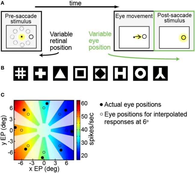
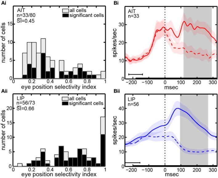
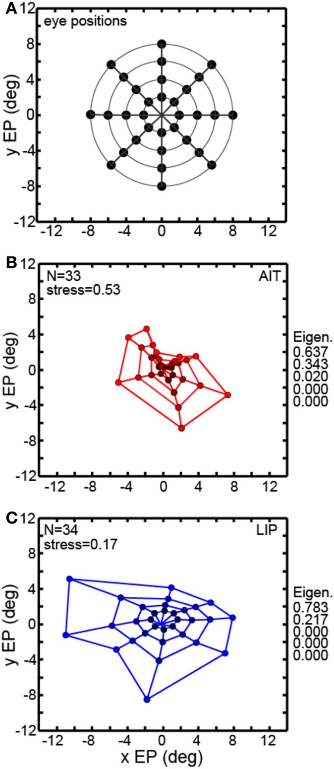
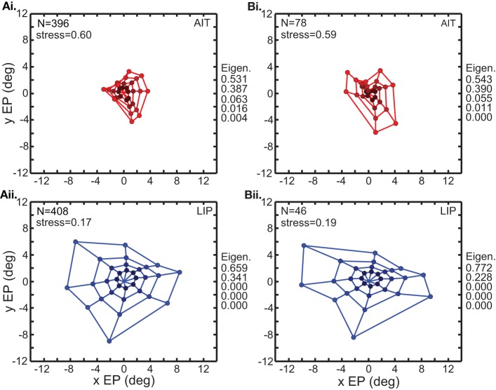
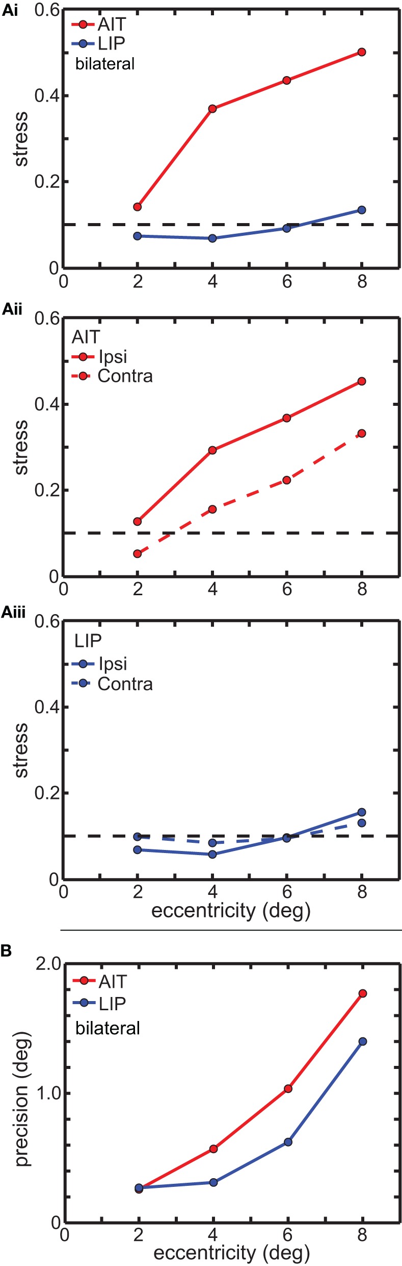
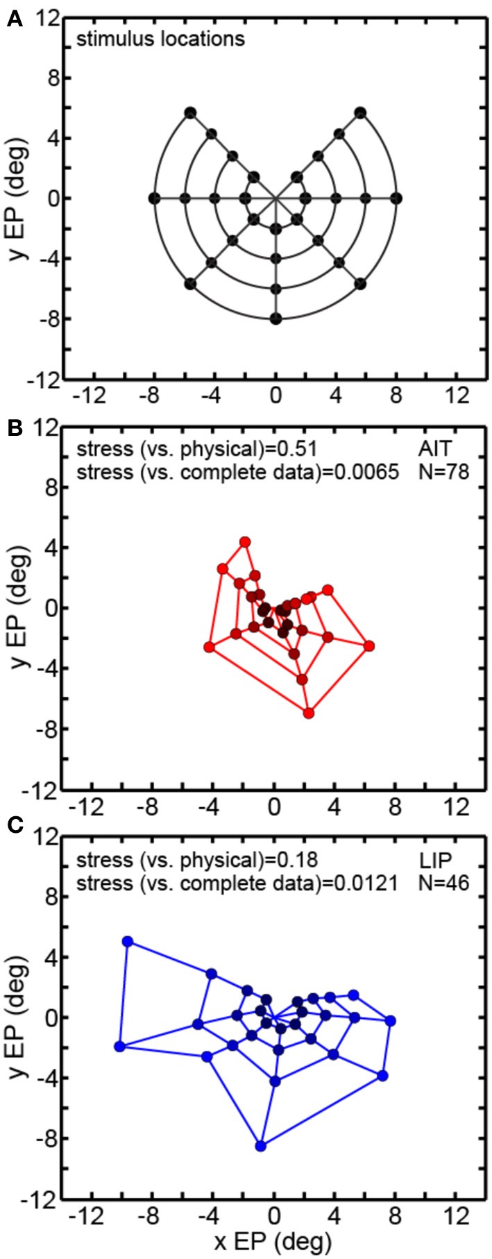
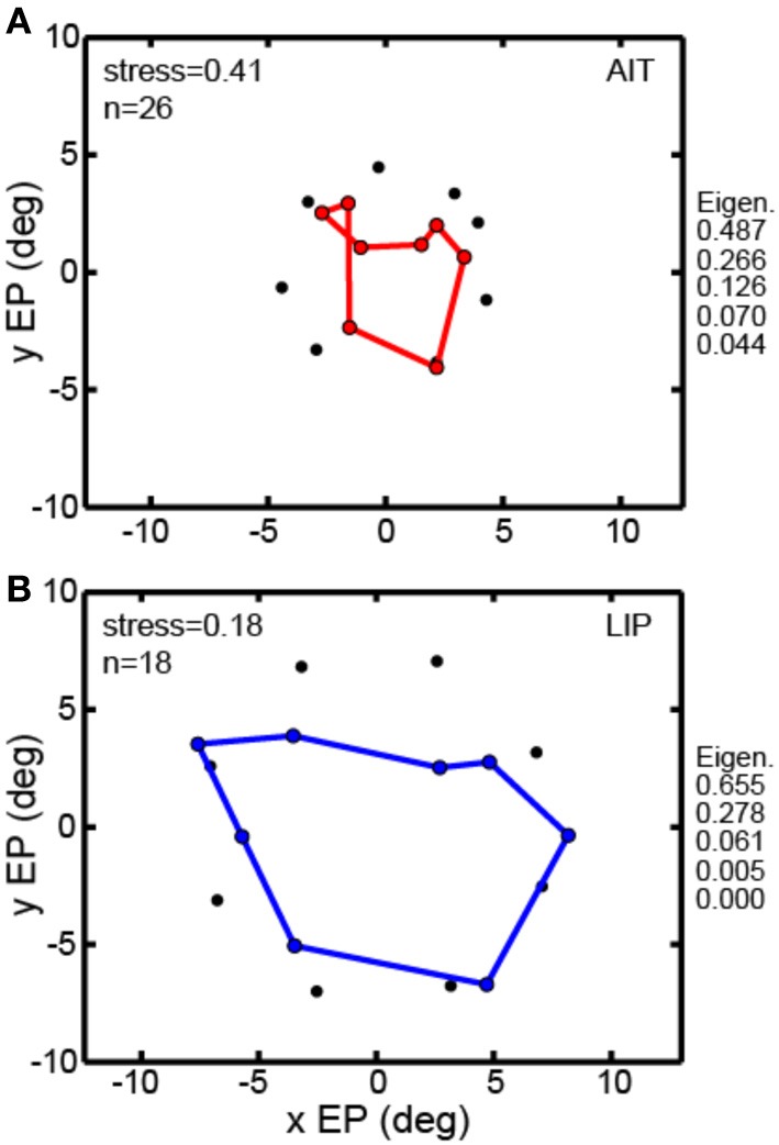
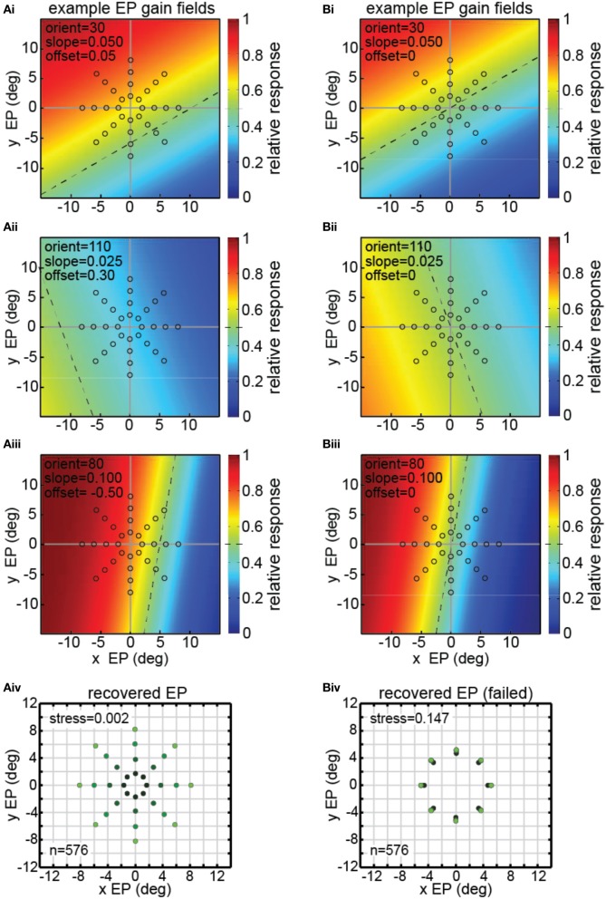
We recorded visual responses while monkeys fixated the same target at different gaze angles, both dorsally (lateral intraparietal cortex, LIP) and ventrally (anterior inferotemporal cortex, AIT). While eye-position modulations occurred in both areas, they were both more frequent and stronger in LIP neurons. We used an intrinsic population decoding technique, multidimensional scaling (MDS), to recover eye positions, equivalent to recovering fixated target locations. We report that eye-position based visual space in LIP was more accurate (i.e., metric). Nevertheless, the AIT spatial representation remained largely topologically correct, perhaps indicative of a categorical spatial representation (i.e., a qualitative description such as "left of" or "above" as opposed to a quantitative, metrically precise description). Additionally, we developed a simple neural model of eye position signals and illustrate that differences in single cell characteristics can influence the ability to recover target position in a population of cells. We demonstrate for the first time that the ventral stream contains sufficient information for constructing an eye-position based spatial representation. Furthermore we demonstrate, in dorsal and ventral streams as well as modeling, that target locations can be extracted directly from eye position signals in cortical visual responses without computing coordinate transforms of visual space.

Keywords: active vision; monkey; multidimensional scaling; population coding; spatial vision.

Figure 1

Experimental and data analysis methods. (A) Task design, showing sequence of events in a single trial. Yellow indicates where the monkey was fixating at each phase of the trial. After the monkey was stably fixating, the stimulus shape appeared randomly at one of eight peripheral locations (first panel). Dotted circles show possible target locations. The monkey immediately made a saccade to the stimulus (second panel). After the saccade (third panel, marked in green) the monkey was stably fixating the target (indicated by the yellow highlight) at some gaze angle. On different trials the target location randomly changed, so we could measure response to the same target stimulus for different eye positions. (B) Set of possible stimulus shapes. Preliminary testing of each cell indicated which of these eight shapes was the most effective stimulus for that cell, which was then used for subsequent measurements of eye-position modulations. (C) Example of interpolated/extrapolated responses used for multidimensional scaling (MDS) analysis, illustrated with data from one cell. Eight filled circles indicate locations where data was collected. Based on those data points an interpolated/extrapolated surface was fit (colored contours), providing an estimate of neural responses to a fixated stimulus over a continuous range of different eye positions. The colored contour map therefore forms a gain field for the cell, providing estimated responses at any arbitrary eye position. Eight open circles are an example set of interpolated/extrapolated eye positions used as input to MDS. Scale bar shows firing rates corresponding to the different colors in the estimated gain field. Only colored regions nearby data locations served as input locations for MDS calculations. That is, as no data came from blanked out regions (polar angles very different from data points, as well as the central area), interpolated values from those regions did not enter into MDS calculations.

Figure 2

Eye position selectivity. (A) Spatial selectivity index (SI) histograms for AIT (upper panel, Ai) and LIP (lower panel, Aii). The SI was calculated for each recorded cell using [Equation (1)]. Included are SI-values for all recorded cells (open bars; second n-value) as well as for only those cells showing significant spatial selectivity (black bars; first n-value). Mean SI-value for spatially significant cells is also shown in each panel indicating the average magnitude of the effects. (B) Average time course of responses (PSTH), aligned to start of saccade to target for AIT (upper panel, Bi, red lines) and LIP (lower panel, Bii, blue lines). Time course calculated over all cells showing significant selectivity for eye position, at the most responsive eye position (solid line) and least responsive eye position (dashed line). Shaded regions around lines show standard errors of responses over cells in the sample population. Zero time marks when the eye left the central fixation window during saccade to target. Black bar at bottom shows target presentation period, with error bar indicating the standard deviation of target onset before saccade to target. Gray shaded region shows the time period used for data analyses (ANOVA, SI, and MDS), beginning 25 ms after start of saccade and ending 200 ms after start of saccade, both times are shifted by the average latency of the visual responses in the respective cortical area.

Figure 3

Recovery of eye positions from neural population activity, using a global stimulus configuration and multidimensional scaling (MDS) analysis. MDS analysis was based on using interpolated neural responses from recorded neurons that had significant spatial selectivity under ANOVA. This analysis used mean neural response across trials. (A) Set of eye positions used as input configuration for MDS analysis. It consisted of 32 points arranged in a polar grid. The center of the grid corresponded to central fixation. As illustrated, the eye positions were arranged over four eccentricities with visual angles of [2°, 4°, 6°, 8°]. At each eccentricity, eight locations were arranged in an iso-centric circle at 45° polar angle increments. Each of the 32 eye positions produced a different activation pattern (response vector) in the population of neurons in our data set. Lines connecting the positions merely help illustrate iso-eccentricity positions and iso-polar angles as well as highlight the overall symmetry of the spatial configuration. (B) Configuration of eye positions recovered from AIT data, shown in red. (C) Configuration of eye positions recovered from LIP data, shown in blue. There is less distortion apparent in the spatial layout of the LIP grid compared to AIT and the LIP stress value is lower than in AIT, indicating a more accurate global recovery of eye positions. For both panels (A) and (B), color darkens with decreasing eccentricity, to aid visualization. Also for both panels, normalized MDS eigenvalues are displayed.

Figure 4

Two variations of the multidimensional scaling analyses in Figure 3. Conventions are the same as in Figure 3, with red points indicating results from AIT and blue points results for LIP. (A) Recovery of eye positions from neural population activity, using single-trial results rather than mean results across trials. Each single-trial response for a given cell was treated in the MDS analysis as a separate cell in the population. (B) Recovery of eye positions from neural population activity, using all cells in the data set rather than only cells that had significant eye-position modulation. Normalized MDS eigenvalues indicated to the right of each panel.

Figure 5

Global and local error measures for multidimensional scaling analysis (MDS) results in Figure 3. (A) Global error (stress) as a function of stimulus eccentricity. Stress values below 0.1 (dashed line in each panel) indicate highly accurate spatial representations. (Ai) Comparison of stress in AIT and LIP using bilateral (ipsilateral and contralateral) data. (Aii) Stress for AIT representations for ipsilateral and contralateral eye positions. (Aiii) Stress for LIP representations for ipsilateral and contralateral eye positions. (B) Local error (precision) as a function of stimulus eccentricity for both AIT (red points) and LIP (blue points). Precision is the standard deviation of recovered eye position, as determined by bootstrap resampling of the data. Precision was individually calculated for each eye position in Figures 3B (AIT) and 3C (LIP), and then for each area averaged over all eye positions having the same eccentricity.

Figure 6

Multidimensional scaling recovery of eye positions using a partial set of inputs. Conventions are the same as in Figure 3. (A) Eye positions used as input configuration for MDS analysis, with one wedge or sector removed compared to the complete set shown in Figure 3A. (B) Configuration of eye positions (red points) recovered from AIT using partial data set. (C) Configuration of eye positions (blue points) recovered from LIP using partial data set. Colors darken at lower eccentricities to aid visualization. Both data panels give stress between recovered eye positions and physical eye positions, as well as stress between recovered eye positions for full and partial data sets. Small stress values between full and partial data indicate that eye position recovery is not highly sensitive to the precise composition of the global configuration used as input to MDS.

Figure 7

Multidimensional scaling recovery of eye positions from population data using the averaging method with a subset of cells rather than interpolation method employed in Figure 3. (A) Configuration of eye positions recovered from AIT (red points). (B) Configuration of eye positions recovered from LIP (blue points). This averaging method replicates the observation found using the interpolation method; namely, that LIP neurons produce a more accurate representation of eye position than AIT (lower stress in LIP than AIT). Normalized MDS eigenvalues indicated to the right of each panel.

Figure 8

Model results showing decoding of eye position, using multidimensional scaling on a population of model neurons with diverse eye-position gain fields. Population consisted of 576 neurons, each with a different gain field. Gain fields were defined by three parameters: slope, orientation, and offset, defined in [Equation (4)]. The color (see scale at right) represents the relative response rate at each eye position. The midpoint firing rate (green) within each gain field (0.5 within the range 0.0–1.0) is shown by a dashed line. (A) Successful decoding of eye position by the model including asymmetric gain fields with large non-zero values of the offset parameter δ = [−1.00, −0.75, −0.50, −0.25, 0.00, 0.25, 0.50, 0.75, 1.00]. (Ai–iii) Three examples of model gain fields with large offsets. Dashed lines do not pass through the origin (central fixation), indicating model neurons included asymmetric gain fields. Open circles indicate eye position locations used as input to MDS analysis, consisting of 32 different eye positions. (Aiv) Multidimensional scaling model results for recovering eye positions, including gain fields with asymmetric gain fields produced using large offsets. Recovered eye positions closely correspond to physical eye positions depicted by open circles in panels (Ai–Aiii). Low stress value indicates the model was able to recover a very accurate representation of relative eye positions. To aid visualization of the spatial configuration of recovered eye positions, the color in the recovered eye position points darkens with decreasing eye position eccentricity. (B) Unsuccessful decoding of eye position by the model using anti-symmetric gain fields produced by small (near zero) offsets (offset parameter, δ = [−0.100, −0.075, −0.050, −0.025, 0.000, 0.025, 0.050, 0.075, 0.100]. (Bi–Biii) Three examples of model gain fields with zero offsets. Dashed lines pass through the origin (central fixation), indicating anti-symmetric gain fields. Open circles indicate spatial locations used as input to MDS analysis, consisting of a stimulus fixated at 32 eye positions. (Biv) MDS modeling results using nearly anti-symmetric gain fields produced using small (near zero) offsets. In this case the model failed to extract accurate eye positions, creating a high stress value, as recovered positions did not closely correspond to physical eye positions depicted by open circles in panels (Bi–Biii) As in (Aiv), color in the recovered eye position points darkens with decreasing eye position eccentricity. In this case, however, the different recovered eye position eccentricities lay nearly on top of each other.

References

1. Aggelopoulos N. C., Rolls E. T. (2005). Scene perception: inferior temporal cortex neurons encode the positions of different objects in the scene. Eur. J. Neurosci. 22, 2903–2916 10.1111/j.1460-9568.2005.04487.x - DOI - PubMed
1. Andersen R. A., Bracewell R. M., Barash S., Gnadt J. W., Fogassi L. (1990). Eye position effects on visual, memory, and saccade-related activity in areas LIP and 7a of macaque. J. Neurosci. 10, 1176–1196 - PMC - PubMed
1. Andersen R. A., Essick G. K., Siegel R. M. (1985). Encoding of spatial location by posterior parietal neurons. Science 230, 456–458 10.1126/science.4048942 - DOI - PubMed
1. Andersen R. A., Mountcastle V. B. (1983). The influence of the angle of gaze upon the excitability of the light-sensitive neurons of the posterior parietal cortex. J. Neurosci. 3, 532–548 - PMC - PubMed
1. Andersen R. A., Snyder L. H., Li C.-S., Stricanne B. (1993). Coordinate transformations in the representation of spatial information. Curr. Opin. Neurobiol. 3, 171–176 10.1016/0959-4388(93)90206-E - DOI - PubMed