An environmental data set for vector-borne disease modeling and epidemiology

Abstract

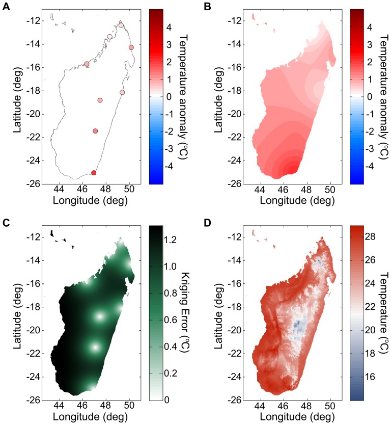
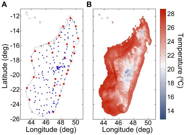
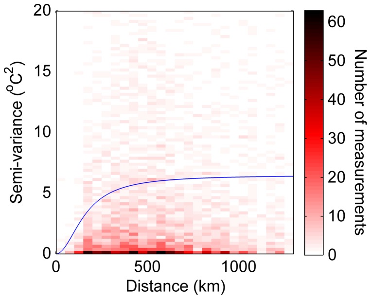
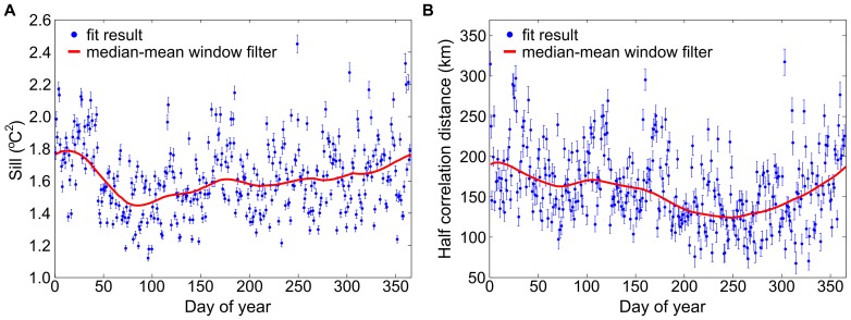
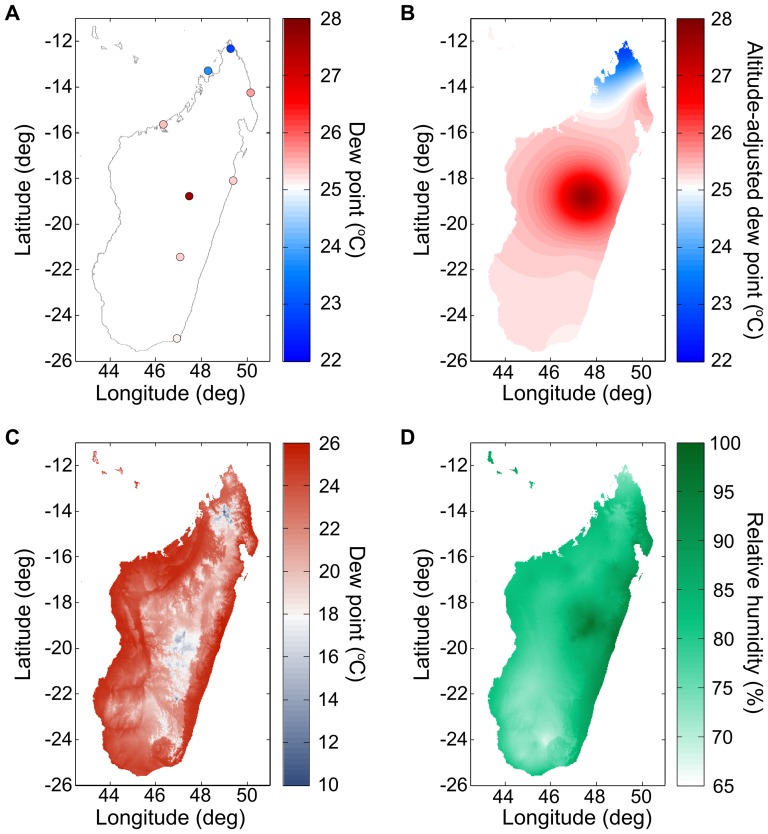
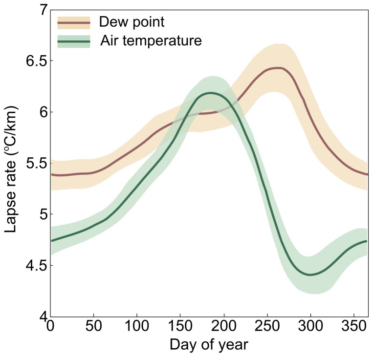
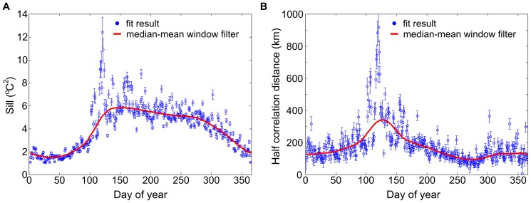
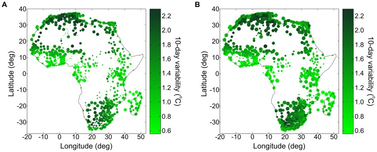
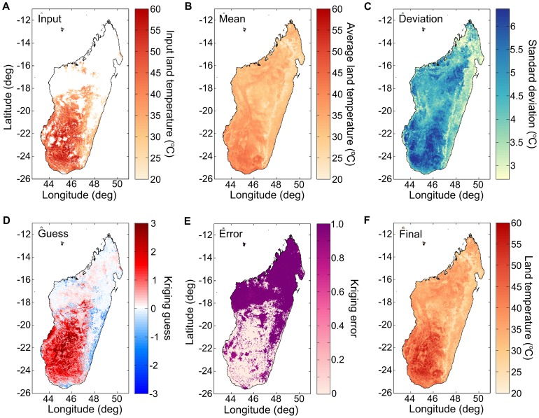
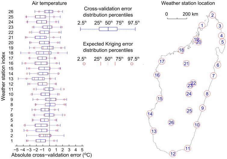
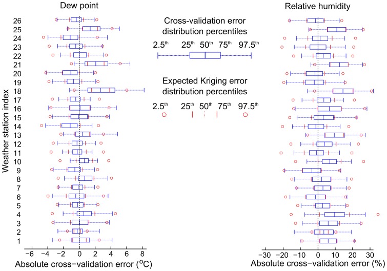
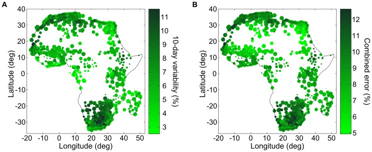
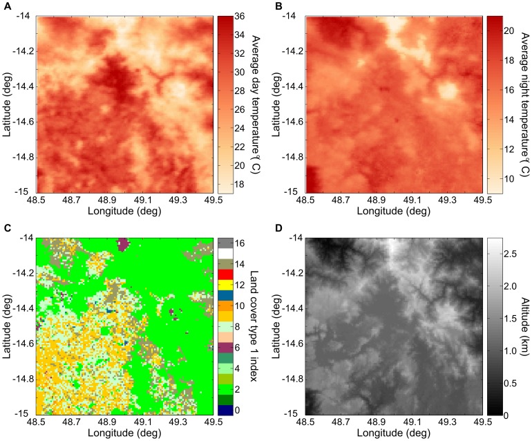
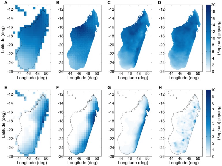
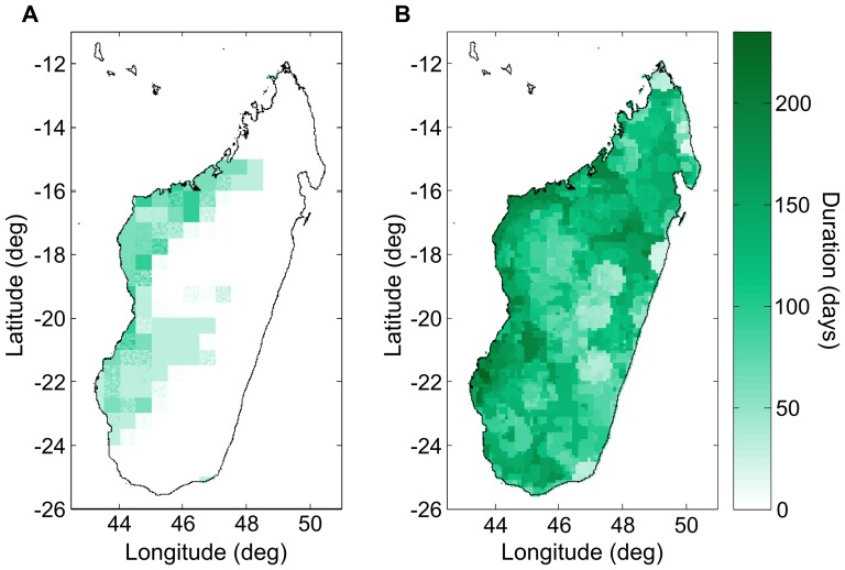
Understanding the environmental conditions of disease transmission is important in the study of vector-borne diseases. Low- and middle-income countries bear a significant portion of the disease burden; but data about weather conditions in those countries can be sparse and difficult to reconstruct. Here, we describe methods to assemble high-resolution gridded time series data sets of air temperature, relative humidity, land temperature, and rainfall for such areas; and we test these methods on the island of Madagascar. Air temperature and relative humidity were constructed using statistical interpolation of weather station measurements; the resulting median 95th percentile absolute errors were 2.75°C and 16.6%. Missing pixels from the MODIS11 remote sensing land temperature product were estimated using Fourier decomposition and time-series analysis; thus providing an alternative to the 8-day and 30-day aggregated products. The RFE 2.0 remote sensing rainfall estimator was characterized by comparing it with multiple interpolated rainfall products, and we observed significant differences in temporal and spatial heterogeneity relevant to vector-borne disease modeling.

Figure 1. Kriging air temperature from Madagascar weather stations.

(A) Extracted air temperature anomalies on January 1^st, 2010. The periodic seasonal components are removed using Fourier transforms. (B) Kriged anomalies across the island and the resulting error estimate (C). The Kriging error increases away from reporting weather stations at the half-correlation distance speed up to the square root of the sill. (D) Combining the WorldClim-derived average temperature surface for that day and the Kriged temperature anomaly, we obtain a prediction of the air temperature throughout the island. In this last image and throughout the data set, the systematical effects of altitude dominate the day-to-day variations due to weather.

Figure 2. Madagascar climate layer.

(A) Weather stations described by Oldeman et al. . The larger red dots are synoptic stations, while the blue dots are simpler field stations. (B) The WorldClim monthly average temperature for January, interpolated from these weather stations .

Figure 3. Example variogram.

Semi-variance of weather station air temperature measurements over Madagascar (1981–2010), for a given day-of-year. The blue curve is the resulting fit of the functional form presented in the Methods section.

Figure 4. Variogram parameters.

Air temperature variogram parameters for Madagascar, from 1981–2010: sill (A) and half correlation distance (B). The blue circles result from fitting the variogram for each day-of-year; the red curve is the smoothed output of the median-mean window filter described in the Methods section and used in our Kriging algorithm.

Figure 5. Calculating relative humidity across Madagascar.

(A) Weather station dew point measurements on January 1^st 2010 (before correcting for altitude). Data from GSOD database .(B) Kriged zero-altitude-equivalent dew point values across the island. (C) Altitude-adjusted Kriged dew point. (D) Combining the Kriged air temperature surface with the dew point surface, to obtain the relative humidity throughout the island.

Figure 6. Lapse rates.

Dew point and air temperature lapse rates in Madagascar, by day of year. The shaded regions represent one standard deviation above and below the median-mean window filter average curve. Note, only the dew point lapse rate is used in the humidity interpolation algorithm.

Figure 7. Variogram parameters.

Dew point variogram parameters for Madagascar, from 1981–2010, by day-of-year: sill (A) and half correlation distance (B). The blue circles result from fitting the variogram for each day-of-year; the red curve is the smooth output of the median-mean window filter described in the Methods section and used in our Kriging algorithm.

Figure 8. Air temperature variability at weather stations across Africa.

Map of the operating weather stations in Africa included in the GSOD database , within (A) the 1981–2000 period and (B) within the 2001–2010 period. Each weather station is represented by a filled circle. Its size is proportional to its reporting frequency (maximum size corresponds to daily reporting), and its color corresponds to the 10-day air-temperature variability. Certain regions of Africa have a dense network of reliable weather stations (e.g. South Africa) while other regions are simply devoid of weather stations (e.g. DRC). Air temperature variability is smallest at the equator (around 0.5°C) and increases up to 2.5°C at 30 degrees of latitude.

Figure 9. Land temperature surface completion method steps.

(A) Remote-sensing measurements of land temperature contain invalid and/or missing pixels (shown in white). The measurements shown here are from the MYD 11A1v005 data set . In order to estimate the land temperate at these missing pixels, the algorithm first calculates the land temperature average (B) and standard deviation (C), for each pixel, for that day of year. At each pixel, the temporal Kriging algorithm then produce a Kriging guesses (D) and a Kriging error (E). Combined with the average of the valid land temperature pixels for that day, a final land temperature surface is constructed (F).

Figure 10. Cross-validation of air temperature Kriging estimates across Madagascar.

(Left) For each weather station, the observed absolute error distribution (blue) is compared with the median error distribution predicted by the Kriging interpolation method (red). The percentiles corresponding to the different features of the boxplot are explained in the legend. (Right) Index of weather station location in Madagascar.

Figure 11. Cross-validation for relative humidity Kriging estimates across Madagascar.

(Left) cross-validation error distributions for dew point, and (right) cross-validation errors for relative humidity. The percentiles corresponding to the different features of the boxplot are explained in the legend.

Figure 12. Relative humidity, 10-day variability, and combined error.

(A) 10-day variability of relative humidity reported by weather stations across Africa (from GSOD database [75]), averaged over the 2001–2010 reporting period. Size of filled circles proportional to the reporting frequency of the station; 10-day variability on a green color scale. (B) By combining the 10-day variability and climate layer error, we obtain a combined average error on relative humidity that is indicative of what the average maximum Kriging error would be.

Figure 13. Daytime and nighttime land surface temperature.

(A–B) Average land surface temperature in a region of Madagascar for January 1^st during the day (at approximately 2 pm) and at night (approximately 2 am) from MODIS aboard the AQUA satellite. (C) Land cover type 1 index classification from the MODIS 12 product . The dominant land cover classification in this region are evergreen broadleaf forest (index 2), savannas (index 9), woody savannas (index 8), barren or sparsely vegetated (index 16), and closed shrubland (index 6). (D) Altitude of the region from the WorldClim data set . Daytime land surface temperature correlates with land cover type; nighttime land surface temperature correlates with altitude.

Figure 14. A comparison of rainfall climate layers.

Average January rainfall across Madagascar according to (A) the CRU2.1 CL (1991–2000) data set , (B) the GPCC (1995–2004) data set , and (C) the WorldClim (1950–2000) data set compared to (D) the average rainfall from the RFE 2.0 (2001–2010) data set . Average July rainfall according to (E) the CRU2.1 CL (1991–2000) data set , (F) the GPCC (1995–2004) data set, and (G) the WorldClim (1950–2000) data set compared to (H) the average rainfall from the RFE 2.0 (2001–2010) data set. There is good agreement between the RFE 2.0 derived climate layer and other established climate layers during the rainy season (e.g., January), but during the dry season (e.g., July) all four climate layers differ, the RFE 2.0 most significantly.

Figure 15. Longest dry spell during a 10-year period.

The (A) GPCC (1995–2004) data set contains significantly shorter dry periods than the (B) RFE 2.0 (2001–2010) data set . In the GPCC time series, any rainfall recorded during a 24 hour period at a weather station extends in the neighboring region (due to spatial interpolation), thus effectively reducing the probability of rain-free day.

References

1. Kiszewski A, Mellinger A, Spielman A, Malaney P, Sachs SE, et al. (2004) A global index representing the stability of malaria transmission. Am J Trop Med Hyg 70: 486–498 Available: http://www.ncbi.nlm.nih.gov/entrez/query.fcgi?cmd=Retrieve&db=PubMed&dop.... - PubMed
1. Sinka ME, Rubio-Palis Y, Manguin S, Patil AP, Temperley WH, et al. (2010) The dominant Anopheles vectors of human malaria in the Americas: occurrence data, distribution maps and bionomic précis. Parasit Vectors 3: 72. - PMC - PubMed
1. Bøgh C, Lindsay SW, Clarke SE, Dean A, Jawara M, et al. (2007) High spatial resolution mapping of malaria transmission risk in the Gambia, west Africa, using LANDSAT TM satellite imagery. Am J Trop Med Hyg 76: 875–881. Available: http://www.ajtmh.org/content/76/5/875.short. Accessed 2013 Nov 19. - PubMed
1. Curran PJ, Atkinson PM, Foody GM, Milton EJ (2000) Linking remote sensing, land cover and disease. Adv Parasitol 47: 37–80. - PubMed
1. Rogers DJ, Hay SI, Packer MJ (1996) Predicting the distribution of tsetse flies in West Africa using temporal Fourier processed meteorological satellite data. Ann Trop Med Parasitol 90: 225–241. - PubMed
Publication types