Emergent global patterns of ecosystem structure and function from a mechanistic general ecosystem model

Abstract

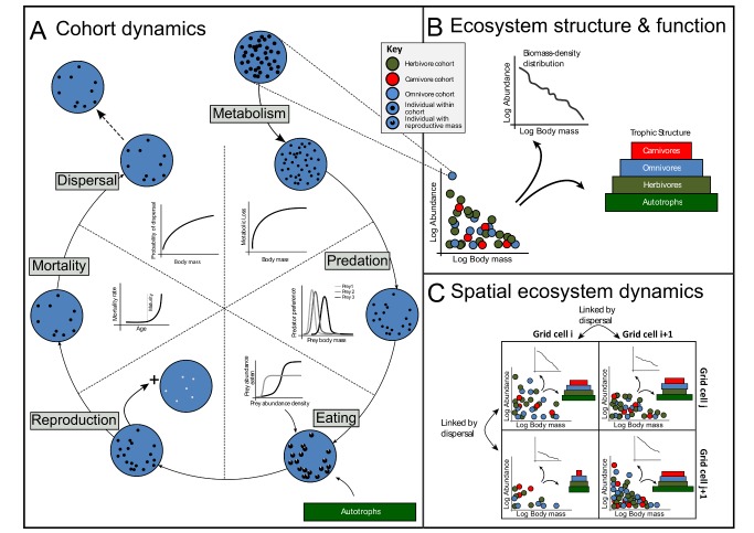
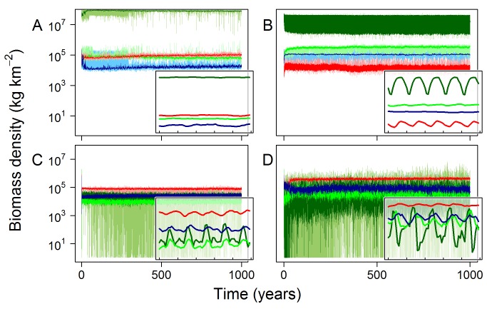
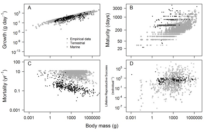
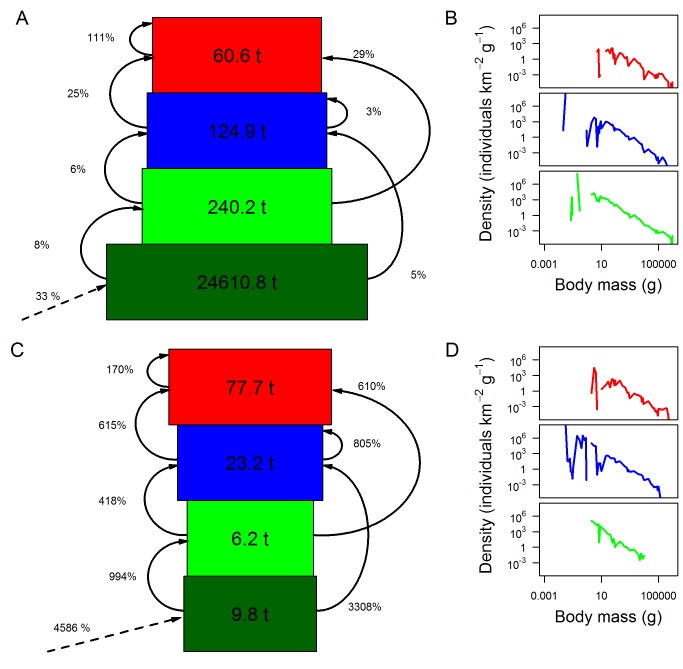
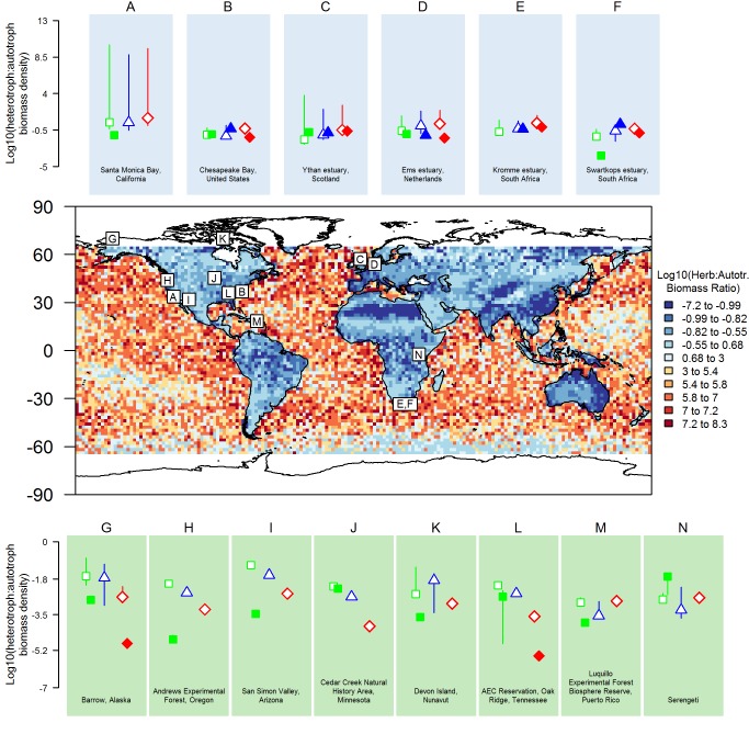
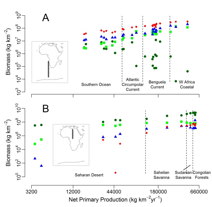
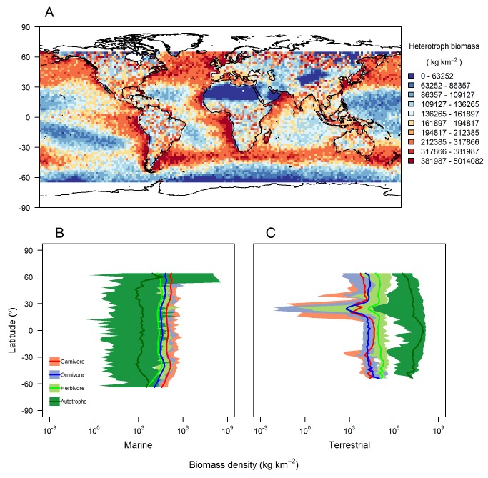
Anthropogenic activities are causing widespread degradation of ecosystems worldwide, threatening the ecosystem services upon which all human life depends. Improved understanding of this degradation is urgently needed to improve avoidance and mitigation measures. One tool to assist these efforts is predictive models of ecosystem structure and function that are mechanistic: based on fundamental ecological principles. Here we present the first mechanistic General Ecosystem Model (GEM) of ecosystem structure and function that is both global and applies in all terrestrial and marine environments. Functional forms and parameter values were derived from the theoretical and empirical literature where possible. Simulations of the fate of all organisms with body masses between 10 µg and 150,000 kg (a range of 14 orders of magnitude) across the globe led to emergent properties at individual (e.g., growth rate), community (e.g., biomass turnover rates), ecosystem (e.g., trophic pyramids), and macroecological scales (e.g., global patterns of trophic structure) that are in general agreement with current data and theory. These properties emerged from our encoding of the biology of, and interactions among, individual organisms without any direct constraints on the properties themselves. Our results indicate that ecologists have gathered sufficient information to begin to build realistic, global, and mechanistic models of ecosystems, capable of predicting a diverse range of ecosystem properties and their response to human pressures.

Figure 1. Schematic of the model.

Ecosystem structure and function (B) emerges from a combination of processes operating on individual organisms within a grid cell (A), and exchange of individuals among grid cells via dispersal (C). Life histories (e.g., average lifespan, lifetime reproductive success, and generation length) are also emergent (not shown in this diagram, but see Figure 3). Fundamental ecological processes affect the ecological properties (principally body mass and abundance; represented as the diameter and number of black dots in A, respectively) of organisms. For computational efficiency, organisms with similar properties are grouped into cohorts (coloured circles in all panels). Graphs in (A) show illustrative examples of functional forms used to model each ecological process; full mathematical details can be found in the main text and in Text S1. Panel (C) illustrates how dispersal links different grid cells through the exchange of cohorts via dispersal. As result of the within-grid-cell processes, and dispersal, the state of the ecosystem—that is, the collection of cohorts within each grid cell—changes dynamically through time. Panel (B) shows two example measures of ecosystem structure that can be calculated at any time: the relative biomasses in different trophic levels, and the body-mass abundance distribution of heterotrophs. All such community-level properties and metrics emerge from bottom-up processes in the model without any model-imposed constraints beyond those processes operating on individual organisms.

Figure 2. 1,000-year dynamics for four locations.

Medians from ensembles of 10 replicate simulations (lines) and absolute ranges (shaded regions) of biomass densities for autotrophs (dark green lines), herbivores (light green), omnivores (blue), and carnivores (red) within four 1°×1° focal grid cells; T1, terrestrial aseasonal (A); T2, terrestrial seasonal (B); M1, marine aseasonal (C); and M2, marine seasonal (D) (Table 4). The temporal dynamics in these metrics emerges from underlying ecological processes that affect a large number of cohorts within each grid cell. Insets zoom in on medians for the last 5 y of the simulations, demonstrating the seasonal variability in each cell.

Figure 3. Comparison of emergent life history metrics with empirical data.

Empirical (black) and emergent model (grey) relationships between body mass and (A) growth rate, (B) maturity, (C) individual mortality rates, and (D) lifetime reproductive success. These life history metrics are not part of the model definition. Rather, they emerge from underlying ecological processes such as metabolism and feeding (see main text). Life history metrics were sampled from 100-y model runs for the four focal grid cells (Table 4). Individual mortality rates are estimated as the inverse of lifespan, and because the minimum simulated lifespan is one model time step (1 mo), estimated individual mortality rates were bounded at 12.

Figure 4. Community-level emergent properties.

Community-level properties—(A, C) biomass pyramids and (B, D) body mass–density relationships across all cohorts belonging to each trophic level—emergent from the model for an example terrestrial (A, B) and marine (C, D) grid cell (grid cells T1 and M1 from Table 4). Results are from the final year of a 100-y model run. Dark green represents autotrophs, light green herbivores, blue omnivores, and red carnivores. In (A) and (C), standing stocks of biomass are indicated by the widths (after log-transformation) and numbers within the boxes; curved arrows and percent values represent the biomass transferred among or within trophic levels from herbivory and predation, as a proportion of the standing stock of the source of each flow; dashed arrows and percent values represent NPP of autotrophs as a proportion of the autotroph standing stock.

Figure 5. Global heterotroph∶autotroph biomass ratios.

Comparisons of modelled (open) and empirical (filled) heterotroph to autotroph biomass ratios in marine (A–F) and terrestrial (G–N) environments (Table S3). Green squares are herbivore to autotroph ratios, blue triangles are omnivore to autotroph ratios, and red diamonds are carnivore to autotroph ratios. Modelled ratios are medians from 10 simulations, and vertical lines are 1 standard deviation over these simulations. Empirical ratios are individual estimates or, where more than one estimate was available, the median of these with sample sizes of H (n = 5), K (n = 2), L (n = 2), and N (n = 3), and vertical lines indicate maximum and minimum empirical estimates. Comparison locations are shown on a map of the predicted ratio of herbivore to autotroph biomass constructed from the global simulation (Study 4, Table 3).

Figure 6. Ecosystem structure along productivity gradients.

Variation in emergent ecosystem structure along productivity gradients in the marine environment (A) from the Southern Ocean to the West African Coast and in the terrestrial realm (B) from the Saharan Desert to the Congolian Forests. Transect locations are presented on the maps set into each panel. Dark green circles correspond to autorotroph biomass, light green squares correspond to herbivore biomass, blue triangles to omnivore biomass, and red diamonds to carnivore biomass. Broad biogeographic regions are roughly distinguished using dashed vertical lines.

Figure 7. Emergent global-level ecosystem properties.

Properties emergent from the model after a 100-y global (65°N to 65°S) simulation using a grid-cell resolution of two degrees. (A) The spatial distribution of annual mean heterotroph biomass density; breaks in the colour scheme were based on quantiles in the data. (B, C) Latitudinal gradients in biomass density; solid lines represent means for each trophic level, and shading represents the range of values across all longitudes in each latitude band.

References

1. Millennium Ecosystem Assessment (2005) Ecosystems and human well-being: biodiversity synthesis. Washington, DC: World Resources Institute.
1. Rodríguez JP, Brotons L, Bustamante J, Seoane J (2007) The application of predictive modelling of species distribution to biodiversity conservation. Divers Distrib 13: 243–251 doi:10.1111/j.1472-4642.2007.00356.x - DOI
1. Thomas CD, Cameron A, Green RE, Bakkenes M, Beaumont LJ, et al. (2004) Extinction risk from climate change. Nature 427: 145–148 doi:10.1038/nature02121 - DOI - PubMed
1. Alkemade R, Oorschot M, Miles L, Nellemann C, Bakkenes M, et al. (2009) GLOBIO3: a framework to investigate options for reducing global terrestrial biodiversity loss. Ecosystems 12: 374–390 doi:10.1007/s10021-009-9229-5 - DOI
1. Mace GM (2013) Ecology must evolve. Nature 503: 191–192. - PubMed
Publication types