Comparison of filtering methods for the modeling and retrospective forecasting of influenza epidemics

Abstract

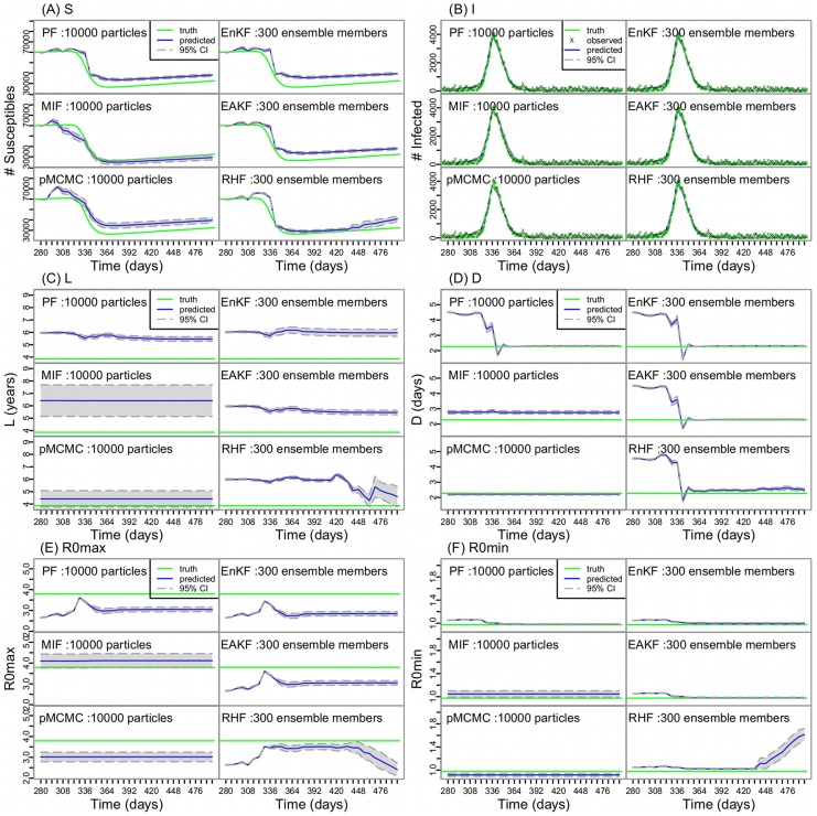
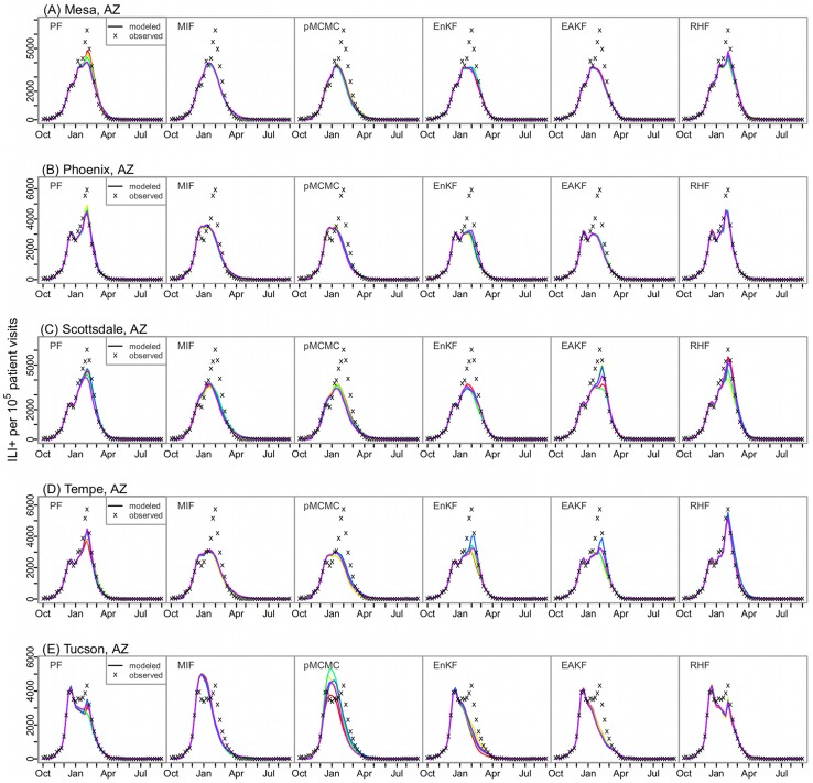
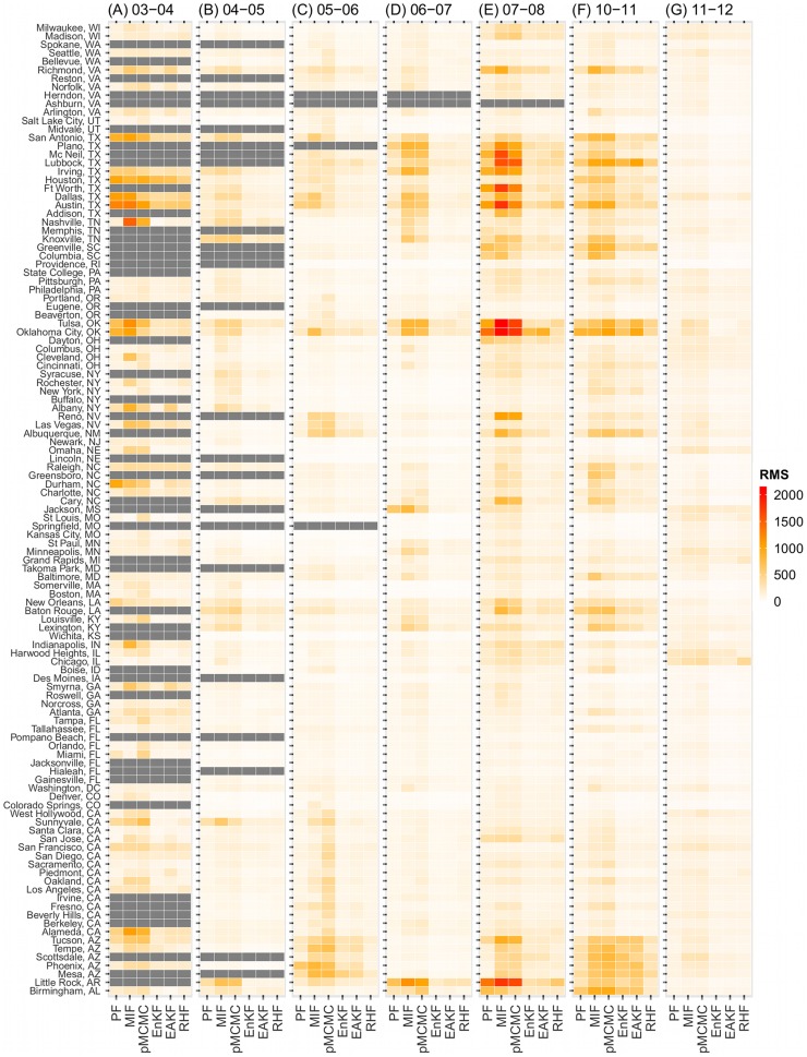
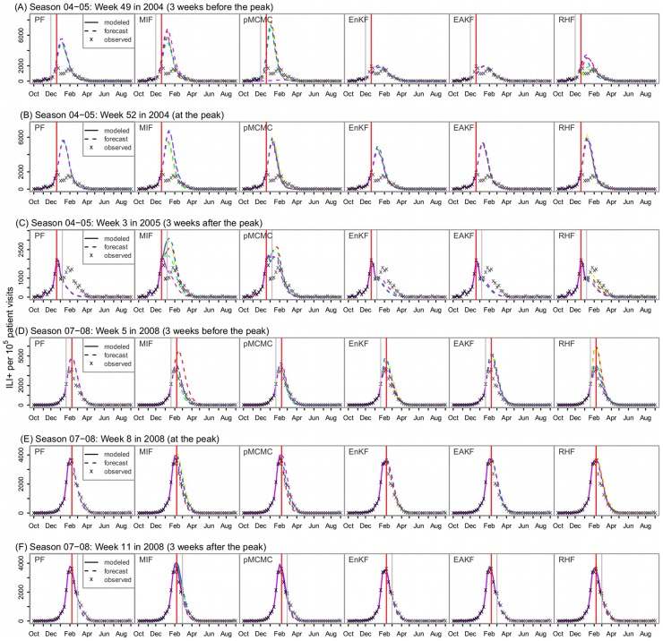
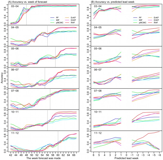
A variety of filtering methods enable the recursive estimation of system state variables and inference of model parameters. These methods have found application in a range of disciplines and settings, including engineering design and forecasting, and, over the last two decades, have been applied to infectious disease epidemiology. For any system of interest, the ideal filter depends on the nonlinearity and complexity of the model to which it is applied, the quality and abundance of observations being entrained, and the ultimate application (e.g. forecast, parameter estimation, etc.). Here, we compare the performance of six state-of-the-art filter methods when used to model and forecast influenza activity. Three particle filters--a basic particle filter (PF) with resampling and regularization, maximum likelihood estimation via iterated filtering (MIF), and particle Markov chain Monte Carlo (pMCMC)--and three ensemble filters--the ensemble Kalman filter (EnKF), the ensemble adjustment Kalman filter (EAKF), and the rank histogram filter (RHF)--were used in conjunction with a humidity-forced susceptible-infectious-recovered-susceptible (SIRS) model and weekly estimates of influenza incidence. The modeling frameworks, first validated with synthetic influenza epidemic data, were then applied to fit and retrospectively forecast the historical incidence time series of seven influenza epidemics during 2003-2012, for 115 cities in the United States. Results suggest that when using the SIRS model the ensemble filters and the basic PF are more capable of faithfully recreating historical influenza incidence time series, while the MIF and pMCMC do not perform as well for multimodal outbreaks. For forecast of the week with the highest influenza activity, the accuracies of the six model-filter frameworks are comparable; the three particle filters perform slightly better predicting peaks 1-5 weeks in the future; the ensemble filters are more accurate predicting peaks in the past.

Figure 1. State estimation using the six filters and synthetic ‘truth’.

The model-filter framework includes two model state variables and four model parameters: (A) the number of susceptible persons S, (B) the number of infected persons I, (C) the immunity period L, (D) the infectious period D, (E) the maximum reproductive number R_0max, and (F) the minimum reproductive number R_0min. The synthetic ‘truth’ for I and S was generated with the SIRS model, for a population of 100,000, with fixed parameters: L = 3.86 y, D = 2.27 d, R_0max = 3.79, and R_0min = 0.97; each model-filter framework was run repeatedly 25 times, with the same set of test data (i.e., synthetic ‘truth’ for the I time series plus random noise, shown as ‘x’ points in (B)). The green lines are the synthetic ‘truth’, blue lines are the mean trajectory over the 25 runs, and the grey areas around them delineate the 95% confidence interval.

Figure 2. ILI+ time series generated from the six filters for New York City.

Simulations are shown for seasons (A) 2003–04, (B) 2004–05, (C) 2005–06, (D) 2006–07, (E) 2007–08, (F) 2010–2011, and (G) 2011–12 (excluding the pandemic seasons). Each model-filter framework was run repeatedly 5 times; each colored line represents one run; the ‘x’ points are the observed weekly ILI+ data.

Figure 3. Fitting multimodal outbreaks.

The model-filter frameworks were tested with historical ILI+ time series collected in the 2010–11 season from 5 cities in Arizona: (A) Mesa, (B) Phoenix, (C) Scottsdale, (D) Tempe, and (E) Tucson; all ILI+ times series had multiple peaks of varying magnitudes; each model-filter framework was run repeatedly 5 times; each colored line represents one run; the ‘x’ points are the observed weekly ILI+ data.

Figure 4. The Root Mean Squared (RMS) error of the six model-filter frameworks used to simulate historical ILI+ for 115 major U.S. cities during the 2003–2012 flu seasons.

Each model-filter framework was run repeatedly 5 times; the RMS error between the predicted and observed ILI+ time series was calculated for each run; the color of each rectangle, corresponding to each city (y-axis) by each filtering framework (x-axis), indicates the average RMS error over the 5 repeated runs for epidemic seasons (A) 2003–04, (B) 2004–05, (C) 2005–06, (D) 2006–07, (E) 2007–08, (F) 2010–2011, and (G) 2011–12.

Figure 5. Predicted ILI+ time series for New York City in the 2004–05 (A–C) and 2007–08 seasons (D–F).

Solid lines (5 lines from five repeated runs for each filter) are modeled based on observations during the training period, and the dashed lines are the forecasts; Red vertical lines indicate the observed peak, and grey vertical lines mark the week the forecasts are made.

Figure 6. Peak timing prediction accuracy.

(A) Accuracy plotted as a function of forecast initiation week; numbers greater than 52/53 weeks are those in the next year, e.g., Week 54 is the first week in 2004 of the 2003–04 season, as 2003 had 53 weeks, and it is the second week in the rest of the seasons; the grey vertical line indicates the peak week most frequently observed among the 115 cities. (B) Accuracy for each predicted lead time with respect to the week of forecast; negative values represent time in the past, e.g., −1 is a peak predicted 1 week in the past. The week 0 predictions are omitted.

Figure 7. Confidence in the prediction.

All forecasts, 565,500 in total, were first categorized according to the mode predicted peak, e.g., 1–3 weeks in the future (the first row) or 3–5 weeks in the past (the last row); within each category, forecasts were further binned by the percentage of ensemble members predicting the mode (PEMPM, e.g., 50–60%) as indicated on the x-axis; the accuracy of forecasts within each bin were then calculated, as shown on the y-axis. The size of the dot in each PEMPM bin indicates the portion of forecasts, within each category, falling into a corresponding bin. Each column (A–F) shows the relationship between the forecast accuracy and the PEMPM for a different filter.

References

1. Molinari N-AM, Ortega-Sanchez IR, Messonnier ML, Thompson WW, Wortley PM, et al. (2007) The annual impact of seasonal influenza in the US: Measuring disease burden and costs. Vaccine 25: 5086–5096. - PubMed
1. Ong JB, Chen MI, Cook AR, Lee HC, Lee VJ, et al. (2010) Real-time epidemic monitoring and forecasting of H1N1-2009 using influenza-like illness from general practice and family doctor clinics in Singapore. PLoS One 5: e10036. - PMC - PubMed
1. Dukic V, Lopes HF, Polson NG (2012) Tracking epidemics with google flu trends data and a state-space SEIR model. Journal of the American Statistical Association 107: 1410–1426. - PMC - PubMed
1. Shaman J, Karspeck A (2012) Forecasting seasonal outbreaks of influenza. Proc Natl Acad Sci USA 109: 20425–20430. - PMC - PubMed
1. Skvortsov A, Ristic B (2012) Monitoring and prediction of an epidemic outbreak using syndromic observations. Mathematical Biosciences 240: 12–19. - PubMed
Publication types